Open Source Statistics with R

Introduction

R is a mature, open-source (i.e. free!) statistics package, with an intuitive interface, excellent graphics and a vibrant community constantly adding new methods for the statistical investigation of your data to the library of packages available.

The goal of this tutorial is to introduce you to the R package, and not to be an introductory course in statistics.

Some excellent examples of using R can also be found at: http://msenux.redwoods.edu/math/R

Getting Started

The very simplest thing we can do with R is to perform some arithmetic at the command prompt:

> phi<-(1+sqrt(5))/2
> phi
[1] 1.618034

Data Structures

Packages

Graphics: A taster

R has some very handy built-in data sets. They allow us to, for example, very simply plot the carbon dioxide concentrations as observed from 1959 to 1997 high above Hawaii at the Mauna Loa observatory.

> plot(pressure)

> plot(co2)

http://www.worldweatheronline.com

> bristol.precip <- c(82.9, 56.1, 59.2, 69, 50.8, 50.9, 50.8, 74.8, 74.7, 91.1, 94.5, 93.6)
> names(bristol.precip) <- c("Jan", "Feb", "Mar", "Apr", "May", "Jun", "Jul", "Aug", "Sep", "Oct", "Nov", "Dec")
> barplot(bristol.precip,
+ main="Average Monthly Precipitation in Bristol",
+ ylab="Mean precipitation (mm)",
+ ylim=c(0,100),
+ col=c("darkblue"))

https://www.gov.uk/government/.../5942-uk-energy-in-brief-2012.pdf‎

> uk.electricty.sources.2011 <- c(41,29,18,5,4,2,1)
> names(uk.electricty.sources.2011) <- ("Gas", "Coal", "Nuclear", "Hydro & other", "Wind", "Imports", "Oil")
> pie(uk.electricty.sources.2011, main="UK Electricty Generating Mix, 2011", col=rainbow(7))

> ?filled.countour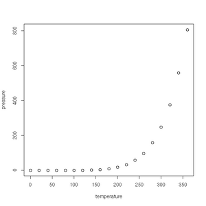

Vapour pressure of mercury against temperature
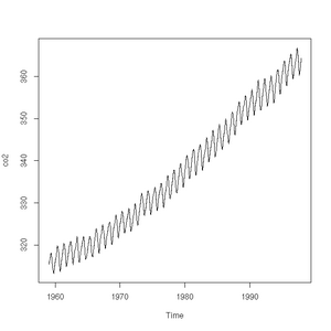
CO2 concentrations measured at Mauna-Loa between 1959 and 1997
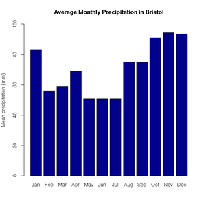
Average monthly precipitation in Bristol

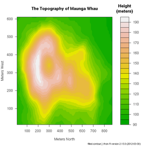
Topology of Maunga Whau volcano in Auckland

Examples of Common Tasks

Linear Regression

> plot(cars)
> res=lm(dist ~ speed, data=cars)
> abline(res)

linear regression of stopping distance against speed from the built-in data set, cars

Exercise

Weighted least squares. The lm function will accept a vector of weights, lm(... weights=...). If given, the function will optimise the line of best fit according a the equation of weighted least squares. Experiment with different linear model fits, given different weighting vectors. Some handy hints for creating a vector of weights:
- w1<-rep(0.1,50) will give you a vector, length 50, where each element has a value of 0.1. W1[1]<-10 will give the first element of the vector a value of 10.
- w2<-seq(from=0.02, to=1.0, by=0.02) provides a vector containing a sequence of values from 0.02 to 1.0 in steps of 0.02 (handily, again 50 in total).

Significance Testing

> boys_2=c(90.2, 91.4, 86.4, 87.6, 86.7, 88.1, 82.2, 83.8, 91, 87.4)
> girls_2=c(83.8, 86.2, 85.1, 88.6, 83, 88.9, 89.7, 81.3, 88.7, 88.4)
> res=var.test(boys_2,girls_2)
> res=t.test(boys_2, girls_2, var.equal=TRUE, paired=FALSE)

R1

Contents