Difference between revisions of "R1"
(→Rmpi) |
|||
| (41 intermediate revisions by the same user not shown) | |||
| Line 8: | Line 8: | ||
The goal of this tutorial is to introduce you to the R package, and not to be an introductory course in statistics. | The goal of this tutorial is to introduce you to the R package, and not to be an introductory course in statistics. | ||
| − | + | If you are working on a Linux system, you will typically start R from the command line. On a Windows machine, or a Mac, you will typically start up R in some form of GUI. However you get R started, you will have access to an R command prompt. The good news is that the examples below will all work at the R command prompt, however you gained access to it. | |
| + | |||
| + | Further resources: | ||
| − | + | * The R manual is a great resource for learning R: http://cran.r-project.org/doc/manuals/r-release/R-intro.pdf | |
| + | * Some excellent examples of using R can also be found at: http://msenux.redwoods.edu/math/R/ and http://www.r-tutor.com/ | ||
=Getting Started= | =Getting Started= | ||
| Line 71: | Line 74: | ||
R also provides '''arrays''', which have more than two dimensions, and '''lists''' to hold heterogeneous collections. | R also provides '''arrays''', which have more than two dimensions, and '''lists''' to hold heterogeneous collections. | ||
| + | |||
| + | An example list: | ||
| + | |||
| + | <source> | ||
| + | > list.r4 <- list(name="Radio4", frequency="93.7") | ||
| + | </source> | ||
| + | |||
| + | The items of which, we can access in several ways: | ||
| + | |||
| + | <source> | ||
| + | > list.r4$frequency | ||
| + | [1] "93.7" | ||
| + | > list.r4[1] | ||
| + | $name | ||
| + | [1] "Radio4" | ||
| + | |||
| + | > list.r4[[1]] | ||
| + | [1] "Radio4" | ||
| + | </source> | ||
A very commonly used data structure is the '''data frame''', which R uses to store tabular data. Given several vectors of equal length, we can collate them into a data frame: | A very commonly used data structure is the '''data frame''', which R uses to store tabular data. Given several vectors of equal length, we can collate them into a data frame: | ||
| Line 85: | Line 107: | ||
2 China 38 27 23 | 2 China 38 27 23 | ||
3 GB 29 17 19 | 3 GB 29 17 19 | ||
| + | </source> | ||
| + | |||
| + | We can access columns of a data frame using the '''$''' operator: | ||
| + | |||
| + | <source> | ||
| + | > medals.2012$country | ||
| + | [1] USA China GB | ||
| + | Levels: China GB USA | ||
| + | > medals.2012$gold | ||
| + | [1] 46 38 29 | ||
</source> | </source> | ||
| Line 111: | Line 143: | ||
<source> | <source> | ||
> uk.electricty.sources.2011 <- c(41,29,18,5,4,2,1) | > uk.electricty.sources.2011 <- c(41,29,18,5,4,2,1) | ||
| − | > names(uk.electricty.sources.2011) <- ("Gas", "Coal", "Nuclear", "Hydro & other", "Wind", "Imports", "Oil") | + | > names(uk.electricty.sources.2011) <- c("Gas", "Coal", "Nuclear", "Hydro & other", "Wind", "Imports", "Oil") |
> pie(uk.electricty.sources.2011, main="UK Electricty Generating Mix, 2011", col=rainbow(7)) | > pie(uk.electricty.sources.2011, main="UK Electricty Generating Mix, 2011", col=rainbow(7)) | ||
</source> | </source> | ||
| Line 149: | Line 181: | ||
</gallery> | </gallery> | ||
| − | There are many more example plots--complete with the R code required to create the plots (at the bottom of the page, after the comments)--on the following web | + | There are many more example plots--complete with the R code required to create the plots (at the bottom of the page, after the comments)--on the following web pages: |
| − | * http://gallery.r- | + | * http://www.sr.bham.ac.uk/~ajrs/R/r-gallery.html |
| + | * http://blog.revolutionanalytics.com/2009/01/r-graph-gallery.html | ||
| + | * https://www.facebook.com/pages/R-Graph-Gallery/169231589826661 | ||
| + | * http://research.stowers-institute.org/efg/R/ | ||
| + | * http://rspatial.r-forge.r-project.org/gallery/ | ||
| + | |||
| + | =Loops= | ||
| + | |||
| + | A simple '''for''' loop: | ||
| + | |||
| + | <source> | ||
| + | > for (ii in seq(1,10)) print(ii) | ||
| + | [1] 1 | ||
| + | [1] 2 | ||
| + | [1] 3 | ||
| + | [1] 4 | ||
| + | [1] 5 | ||
| + | [1] 6 | ||
| + | [1] 7 | ||
| + | [1] 8 | ||
| + | [1] 9 | ||
| + | [1] 10 | ||
| + | </source> | ||
| + | |||
| + | Some more exotic counting: | ||
| + | |||
| + | <source> | ||
| + | > for (ii in seq(from=10, to=0, by=-2)) print(ii) | ||
| + | [1] 10 | ||
| + | [1] 8 | ||
| + | [1] 6 | ||
| + | [1] 4 | ||
| + | [1] 2 | ||
| + | [1] 0 | ||
| + | </source> | ||
| + | |||
| + | '''while''' loops are for when we don't know the number of iterations in advance: | ||
| + | |||
| + | <source> | ||
| + | > ii <- runif(1,0,1) | ||
| + | > ii | ||
| + | [1] 0.3998513 | ||
| + | > while (ii < 0.5) {print(ii); ii <- runif(1,0,1)} | ||
| + | [1] 0.3998513 | ||
| + | [1] 0.05469244 | ||
| + | > ii | ||
| + | [1] 0.8265036 | ||
| + | </source> | ||
=Functions= | =Functions= | ||
| Line 216: | Line 295: | ||
Listed at http://cran.r-project.org/ | Listed at http://cran.r-project.org/ | ||
| − | Let's install the ''' | + | Let's install the '''GoogleVis''' package, that provides an interface between R and Google Charts. Google Charts offer interactive charts which can be embedded into web pages. The best known of these charts is probably the Motion Chart, popularised by Hans Rosling in his TED talks. (See http://cran.r-project.org/web/packages/googleVis/vignettes/googleVis.pdf for more information on this package.) |
<source> | <source> | ||
| − | > install.packages(" | + | > install.packages("googleVis") |
</source> | </source> | ||
| Line 233: | Line 312: | ||
<source> | <source> | ||
| − | > library( | + | > library(googleVis) |
</source> | </source> | ||
| − | + | Another package you might like to try is '''xlsx''' package for reading/writing MS Excel files (http://cran.r-project.org/web/packages/xlsx/vignettes/xlsx.pdf). | |
| − | |||
| − | |||
| − | |||
| − | |||
| − | |||
| − | |||
| − | |||
| − | |||
| − | |||
| − | |||
| − | |||
| − | |||
| − | |||
| − | |||
| − | |||
| − | |||
| − | |||
| − | |||
| − | |||
| − | |||
| − | |||
| − | |||
| − | |||
=Reading Data from File= | =Reading Data from File= | ||
| Line 348: | Line 404: | ||
=Examples of Common Tasks= | =Examples of Common Tasks= | ||
| + | |||
| + | ==Preparing Data== | ||
| + | |||
| + | ===Sorting=== | ||
| + | |||
| + | Using '''sort''': | ||
| + | |||
| + | <source> | ||
| + | > railway.engines <- c("thomas", "henry", "gordon", "edward", "james") | ||
| + | > sort(railway.engines) | ||
| + | [1] "edward" "gordon" "henry" "james" "thomas" | ||
| + | </source> | ||
| + | |||
| + | See: http://stat.ethz.ch/R-manual/R-devel/library/base/html/sort.html | ||
| + | |||
| + | ===Random Sampling=== | ||
| + | |||
| + | Using '''sample''': | ||
| + | |||
| + | <source> | ||
| + | > railway.engines <- c("thomas", "henry", "gordon", "edward", "james") | ||
| + | > sample(railway.engines, 1, replace = TRUE, prob = NULL) | ||
| + | [1] "gordon" | ||
| + | > sample(railway.engines, 1, replace = TRUE, prob = NULL) | ||
| + | [1] "james" | ||
| + | > sample(railway.engines, 1, replace = TRUE, prob = NULL) | ||
| + | [1] "edward" | ||
| + | > sample(railway.engines, 1, replace = TRUE, prob = NULL) | ||
| + | [1] "thomas" | ||
| + | > sample(railway.engines, 1, replace = TRUE, prob = NULL) | ||
| + | [1] "gordon" | ||
| + | > sample(railway.engines, 1, replace = TRUE, prob = NULL) | ||
| + | [1] "james" | ||
| + | </source> | ||
| + | |||
| + | See: http://stat.ethz.ch/R-manual/R-devel/library/base/html/sample.html | ||
| + | |||
| + | ===Combining=== | ||
| + | |||
| + | Using '''rbind''' to add combine the rows to two data frames: | ||
| + | |||
| + | <source> | ||
| + | > country <- c("France", "Italy", "Hungary", "Australia") | ||
| + | > gold <- c(11, 8, 8, 7) | ||
| + | > silver <- c(11, 9, 4, 16) | ||
| + | > bronze <- c(12, 11, 5, 12) | ||
| + | > extras.2012 <- data.frame(country, gold, silver, bronze) | ||
| + | > rbind(medals.2012, extras.2012) | ||
| + | country gold silver bronze | ||
| + | 1 USA 46 29 29 | ||
| + | 2 China 38 27 23 | ||
| + | 3 Great Britain 29 17 19 | ||
| + | 4 Russian Federation 24 26 32 | ||
| + | 5 Republic of Korea 13 8 7 | ||
| + | 6 Germany 11 19 14 | ||
| + | 7 France 11 11 12 | ||
| + | 8 Italy 8 9 11 | ||
| + | 9 Hungary 8 4 5 | ||
| + | 10 Australia 7 16 12 | ||
| + | </source> | ||
| + | |||
| + | See: http://stat.ethz.ch/R-manual/R-devel/library/base/html/cbind.html | ||
| + | |||
| + | ===Binning Data=== | ||
| + | |||
| + | Using '''cut''': | ||
| + | |||
| + | <source> | ||
| + | > girls_2=c(83.8, 86.2, 85.1, 88.6, 83, 88.9, 89.7, 81.3, 88.7, 88.4) | ||
| + | > bins=cut(girls_2, breaks=3) | ||
| + | > bins | ||
| + | [1] (81.3,84.1] (84.1,86.9] (84.1,86.9] (86.9,89.7] (81.3,84.1] (86.9,89.7] | ||
| + | [7] (86.9,89.7] (81.3,84.1] (86.9,89.7] (86.9,89.7] | ||
| + | Levels: (81.3,84.1] (84.1,86.9] (86.9,89.7] | ||
| + | > plot(bins) | ||
| + | </source> | ||
| + | |||
| + | Plotting the data couldn't be simpler with '''plot(bins)'''! | ||
| + | |||
| + | See: http://stat.ethz.ch/R-manual/R-devel/library/base/html/cut.html | ||
==Linear Regression== | ==Linear Regression== | ||
| Line 361: | Line 497: | ||
---- | ---- | ||
| − | ''' | + | '''Exercises''' |
| + | * You may wish to compare different methods of estimation. From the MASS package, you can fit a line with the '''rlm''' and '''lqs'' funtions. You can plot all the lines against the data using: | ||
| + | <source> | ||
| + | > abline(res.lm, lty=1) | ||
| + | > abline(res.rlm, lty=2) | ||
| + | > abline(res.lqs, lty=3) | ||
| + | > legend(x=5, y=100, legend=c("lm","rlm","lqs"), lty=c(1,2,3)) | ||
| + | </source> | ||
| + | See: http://stat.ethz.ch/R-manual/R-patched/library/MASS/html/rlm.html and http://stat.ethz.ch/R-manual/R-devel/RHOME/library/MASS/html/lqs.html. | ||
| + | |||
* Weighted least squares. The '''lm''' function will accept a vector of weights, '''lm(... weights=...)'''. If given, the function will optimise the line of best fit according a the equation of weighted least squares. Experiment with different linear model fits, given different weighting vectors. Some handy hints for creating a vector of weights: | * Weighted least squares. The '''lm''' function will accept a vector of weights, '''lm(... weights=...)'''. If given, the function will optimise the line of best fit according a the equation of weighted least squares. Experiment with different linear model fits, given different weighting vectors. Some handy hints for creating a vector of weights: | ||
** '''w1<-rep(0.1,50)''' will give you a vector, length 50, where each element has a value of 0.1. W1[1]<-10 will give the first element of the vector a value of 10. | ** '''w1<-rep(0.1,50)''' will give you a vector, length 50, where each element has a value of 0.1. W1[1]<-10 will give the first element of the vector a value of 10. | ||
| Line 399: | Line 544: | ||
</source> | </source> | ||
| − | = | + | ==Classification== |
| − | + | ===k Nearest Neighbours=== | |
| − | + | This famous (Fisher's or Anderson's) iris data set gives the measurements in centimeters of the variables sepal length and width and petal length and width, respectively, for 50 flowers from each of 3 species of iris. The species are Iris setosa (s), versicolor (c), and virginica (v). | |
| − | + | See: http://stat.ethz.ch/R-manual/R-patched/library/datasets/html/iris.html | |
| − | + | k-nearest neighbour classification for test set from training set: For each row of the test set, the k nearest (in Euclidean distance) training set vectors are found, and the classification is decided by majority vote, with ties broken at random. If there are ties for the kth nearest vector, all candidates are included in the vote. | |
| + | |||
| + | See: http://stat.ethz.ch/R-manual/R-devel/library/class/html/knn.html | ||
| − | |||
<source> | <source> | ||
| − | library( | + | library(class) |
| − | + | train <- rbind(iris3[1:25,,1], iris3[1:25,,2], iris3[1:25,,3]) | |
| − | + | test <- rbind(iris3[26:50,,1], iris3[26:50,,2], iris3[26:50,,3]) | |
| − | + | cl <- factor(c(rep("s",25), rep("c",25), rep("v",25))) | |
| − | + | iris3.knn <- knn(train, test, cl, k = 3, prob=TRUE) | |
| − | + | table(predicted=iris3.knn, actual=cl) | |
| − | |||
| − | |||
| − | |||
</source> | </source> | ||
| − | + | How did we do? | |
| − | |||
| − | |||
| − | |||
| − | |||
| − | |||
| − | |||
| − | |||
| − | |||
| − | |||
| − | |||
| − | |||
| − | |||
| − | |||
| − | |||
| − | |||
<pre> | <pre> | ||
| − | + | actual | |
| − | + | predicted c s v | |
| − | + | c 23 0 3 | |
| − | + | s 0 25 0 | |
| − | + | v 2 0 22 | |
| − | |||
| − | |||
| − | |||
| − | |||
| − | |||
| − | |||
| − | |||
| − | |||
| − | |||
</pre> | </pre> | ||
| − | == | + | ===Classification Trees=== |
| − | |||
| − | |||
| − | |||
| − | |||
| − | |||
| − | |||
| − | |||
| − | |||
| − | |||
| − | |||
| − | |||
| − | |||
| − | |||
| − | |||
| − | |||
| − | |||
| − | |||
| − | |||
| − | |||
| − | |||
| − | |||
| − | |||
| − | |||
| − | |||
| − | |||
| − | |||
| − | |||
| − | |||
| − | |||
| − | |||
| − | |||
| − | |||
| − | |||
| − | |||
| − | |||
| − | |||
| − | |||
| − | |||
| − | |||
| − | |||
| − | |||
| − | |||
| − | |||
| − | |||
| − | |||
| − | |||
| − | |||
| − | |||
| − | |||
| − | |||
| − | |||
| − | |||
| − | |||
| − | |||
| − | |||
| − | + | The kyphosis data frame has 81 rows and 4 columns. representing data on children who have had corrective spinal surgery. | |
| − | |||
| − | + | This data frame contains the following columns: | |
| − | + | * Kyphosis: a factor with levels absent present indicating if a kyphosis (a type of deformation) was present after the operation. | |
| − | + | * Age: in months | |
| − | + | * Number: the number of vertebrae involved | |
| − | + | * Start: the number of the first (topmost) vertebra operated on. | |
| − | |||
| − | |||
| − | + | See: http://stat.ethz.ch/R-manual/R-devel/library/rpart/html/kyphosis.html | |
| − | |||
<source> | <source> | ||
| − | + | fit <- rpart(Kyphosis ~ Age + Number + Start, data = kyphosis) | |
| − | + | fit2 <- rpart(Kyphosis ~ Age + Number + Start, data = kyphosis, | |
| − | + | parms = list(prior = c(.65,.35), split = "information")) | |
| − | + | fit3 <- rpart(Kyphosis ~ Age + Number + Start, data = kyphosis, | |
| − | + | control = rpart.control(cp = 0.05)) | |
| − | + | par(mfrow = c(1,2), xpd = NA) # otherwise on some devices the text is clipped | |
| − | + | plot(fit) | |
| − | + | text(fit, use.n = TRUE) | |
| − | + | plot(fit2) | |
| − | + | text(fit2, use.n = TRUE) | |
| − | |||
</source> | </source> | ||
| − | + | [[Image:R-classification-tree.png|500px|thumbnail|center|Classification tree for the kyphosis data frame.]] | |
| − | |||
| − | |||
| − | |||
| − | |||
| − | |||
| − | |||
| − | |||
| − | |||
| − | |||
| − | + | ==Solving Systems of Linear Equations== | |
| − | |||
| − | |||
| − | |||
| − | |||
| − | |||
| − | |||
| − | |||
| − | |||
| − | |||
| − | |||
| − | |||
| − | |||
| − | |||
| − | |||
| − | |||
| − | |||
| − | |||
| − | |||
| − | |||
| − | + | See, e.g.: https://source.ggy.bris.ac.uk/wiki/NumMethodsPDEs | |
| − | |||
<source> | <source> | ||
| − | + | > A <- array(c(1,3,2,3,5,4,-2,6,3), dim=c(3,3)) | |
| − | + | > b <- c(5,7,8) | |
| − | + | > solve(A,b) | |
| − | + | [1] -15 8 2 | |
| − | |||
| − | |||
| − | |||
| − | |||
| − | |||
</source> | </source> | ||
| − | + | =Suggested Exercises= | |
| − | + | If you would like to work through some exercises, with model answers included, you could take a look at: | |
| + | * http://www2.warwick.ac.uk/fac/sci/statistics/staff/academic-research/reed/rexercises.pdf | ||
| − | * | + | If you would prefer to noodle about with some real-world data, you could take a look at: |
| − | + | * http://www.theguardian.com/news/datablog/2010/oct/18/historic-government-spending-area#data | |
Latest revision as of 17:06, 10 December 2014
Open Source Statistics with R
Introduction
R is a mature, open-source (i.e. free!) statistics package, with an intuitive interface, excellent graphics and a vibrant community constantly adding new methods for the statistical investigation of your data to the library of packages available.
The goal of this tutorial is to introduce you to the R package, and not to be an introductory course in statistics.
If you are working on a Linux system, you will typically start R from the command line. On a Windows machine, or a Mac, you will typically start up R in some form of GUI. However you get R started, you will have access to an R command prompt. The good news is that the examples below will all work at the R command prompt, however you gained access to it.
Further resources:
- The R manual is a great resource for learning R: http://cran.r-project.org/doc/manuals/r-release/R-intro.pdf
- Some excellent examples of using R can also be found at: http://msenux.redwoods.edu/math/R/ and http://www.r-tutor.com/
Getting Started
The very simplest thing we can do with R is to perform some arithmetic at the command prompt:
> phi <- (1+sqrt(5))/2
> phi
[1] 1.618034
Parentheses are used to modify the usual order of precedence of the operators (/ will typically be evaluated before +). Note the [1] accompanying the returned value. All numbers entered at the console are interpreted as a vector. The '[1]' indicates that the line in question is displaying the vector of values starting at first index. We can use the handy sequence function to create a vector containing more than a single element:
> odds <- seq(from=1, to=67, by=2)
> odds
 [1]  1  3  5  7  9 11 13 15 17 19 21 23 25 27 29 31 33 35 37 39 41 43 45 47 49
[26] 51 53 55 57 59 61 63 65 67
From the above example, we can see that both the <- and = operators can be used for assignment.
Vectors are commonly used data structures in R:
coords.bris <- c(51.5, 2.6)As are matrices:
> magic <- matrix(data=c(2,7,6,9,5,1,4,3,8),nrow=3,ncol=3)
> magic
     [,1] [,2] [,3]
[1,]    2    9    4
[2,]    7    5    3
[3,]    6    1    8
Where the c function combines the arguments given in the parentheses. We can access portions of the array using the syntax shown in the square brackets. For example, we can access the first row using the [1,] notation, and similarly the second column using [,2]. Since the square is 3x3 magic, the numbers in both slices should sum to 15:
> sum(magic[1,])
[1] 15
> sum(magic[,2])
[1] 15
Single elements and ranges can also accessed:
> magic[2,2]
[1] 5
> magic[2:3,2:3]
     [,1] [,2]
[1,]    5    3
[2,]    1    8
R also provides arrays, which have more than two dimensions, and lists to hold heterogeneous collections.
An example list:
> list.r4 <- list(name="Radio4", frequency="93.7")The items of which, we can access in several ways:
> list.r4$frequency
[1] "93.7"
> list.r4[1]
$name
[1] "Radio4"

> list.r4[[1]]
[1] "Radio4"
A very commonly used data structure is the data frame, which R uses to store tabular data. Given several vectors of equal length, we can collate them into a data frame:
> country <- c("USA", "China", "GB")
> gold <- c(46, 38, 29)
> silver <- c(29, 27, 17)
> bronze <- c(29, 23, 19)
> medals.2012 <- data.frame(country, gold, silver, bronze)
> medals.2012
    country  gold  silver  bronze
1       USA    46      29      29
2     China    38      27      23
3        GB    29      17      19
We can access columns of a data frame using the $ operator:
> medals.2012$country
[1] USA   China GB
Levels: China GB USA
> medals.2012$gold
[1] 46 38 29
Standard Graphics: A taster
An aspect which makes R popular are it's graphing functions. R also has some very handy built-in data sets--we'll use this to demonstrate just a small fraction of R's graphing abilities.
First up is the humble plot() function. Given a data frame of points, such as one charting the relationship between temperature and the vapour pressure of mercury, it will give us a (handily labelled) scatter plot:
> plot(pressure)See the gallery below for all the plots created in this section.
The plot function will also accept a time-series (another class of object recognised by R) and will sensibly join the points with a line:
> plot(co2)
> class(co2)
[1] "ts"
Pie charts are easily constructed. In this case, to show the relative proportions of electricity generated from different sources in the UK in 2011 (source: https://www.gov.uk/government/.../5942-uk-energy-in-brief-2012.pdf):
> uk.electricty.sources.2011 <- c(41,29,18,5,4,2,1)
> names(uk.electricty.sources.2011) <- c("Gas", "Coal", "Nuclear", "Hydro & other", "Wind", "Imports", "Oil")
> pie(uk.electricty.sources.2011, main="UK Electricty Generating Mix, 2011", col=rainbow(7))
Next, let's create a bar chart of monthly average precipitation falling here in the fair city of Bristol (source: http://www.worldweatheronline.com):
> bristol.precip <- c(82.9, 56.1, 59.2, 69, 50.8, 50.9, 50.8, 74.8, 74.7, 91.1, 94.5, 93.6)
> names(bristol.precip) <- c("Jan", "Feb", "Mar", "Apr", "May", "Jun", "Jul", "Aug", "Sep", "Oct", "Nov", "Dec")
> barplot(bristol.precip,
+ main="Average Monthly Precipitation in Bristol",
+ ylab="Mean precipitation (mm)",
+ ylim=c(0,100),
+ col=c("darkblue"))
'Box and whisker' plots are useful ways to graph the quartiles of some data. In this case, the fuel efficiencies of various US cars, circa 1974:
> boxplot(mpg~cyl,data=mtcars, main="Car Milage Data",
+    xlab="Number of Cylinders", ylab="Miles Per Gallon")
R includes a very useful help facility. In the case of the filled.contour() plotting function, the help page includes an example of it's use to plot the topology of a volcano in Auckland, NZ:
> ?filled.countour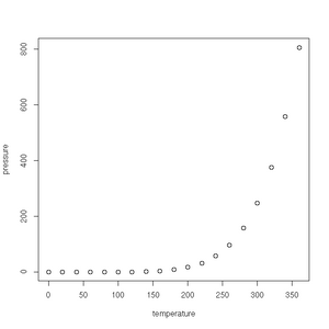
Vapour pressure of mercury against temperature
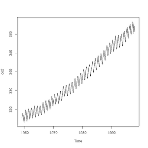
CO2 concentrations measured at Mauna-Loa between 1959 and 1997
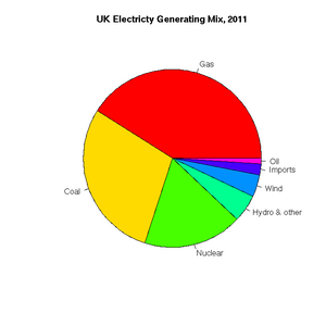
The UK's electricity generating mix, 2011
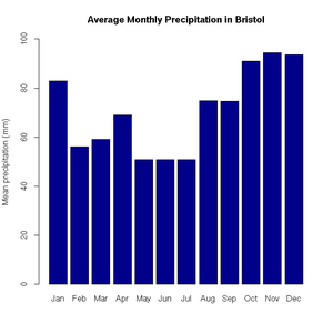
Average monthly precipitation in Bristol
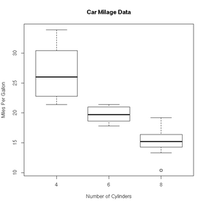
Range of fuel efficiencies for different engine sizes
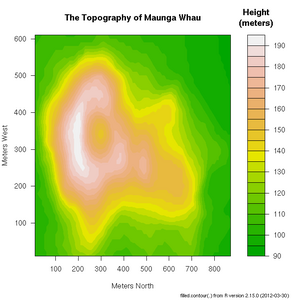
Topology of Maunga Whau volcano in Auckland


There are many more example plots--complete with the R code required to create the plots (at the bottom of the page, after the comments)--on the following web pages:
- http://www.sr.bham.ac.uk/~ajrs/R/r-gallery.html
- http://blog.revolutionanalytics.com/2009/01/r-graph-gallery.html
- https://www.facebook.com/pages/R-Graph-Gallery/169231589826661
- http://research.stowers-institute.org/efg/R/
- http://rspatial.r-forge.r-project.org/gallery/
Loops
A simple for loop:
> for (ii in seq(1,10)) print(ii)
[1] 1
[1] 2
[1] 3
[1] 4
[1] 5
[1] 6
[1] 7
[1] 8
[1] 9
[1] 10
Some more exotic counting:
> for (ii in seq(from=10, to=0, by=-2)) print(ii)
[1] 10
[1] 8
[1] 6
[1] 4
[1] 2
[1] 0
while loops are for when we don't know the number of iterations in advance:
> ii <- runif(1,0,1)
> ii
[1] 0.3998513
> while (ii < 0.5) {print(ii); ii <- runif(1,0,1)}
[1] 0.3998513
[1] 0.05469244
> ii
[1] 0.8265036
Functions
You can define your own functions in R, using the function keyword. For example, Pythagoras' Theorem:
> hypotenuse <- function(x, y) {sqrt(x^2 + y^2)}The braces ({}) are optional, but add clarity.
To call the function:
> hypotenuse(3,4)
[1] 5
We can provide default values for the arguments, which can be overridden for any given invocation of the function:
> hypot2 <- function(x=3 ,y=4) {sqrt(x^2 + y^2)}
> hypot2()
[1] 5
> hypot2(12,16)
[1] 20
> hypot2(y=16, x=12)
[1] 20
You can see that the order of the arguments is respected, unless the names are given, in which case the order can be changed.
Longer functions can be spread over several lines. We can also use the return keyword to control which value is returned by the function:
> hypot3 <- function(x=3 ,y=4) {
+ x_sq <- x^2
+ y_sq <- y^2
+ return( sqrt(x_sq + y_sq) )}
> hypot3(6,8)
[1] 10
You can check on the contents of a function, by just typing it's name (without parentheses):
> hypot3
function(x=3 ,y=4) {
x_sq <- x^2
y_sq <- y^2
return( sqrt(x_sq + y_sq) )}
Or just check the arguments, using the args function. (The body of the function in general is reported as NULL):
> args(hypot3)
function (x = 3, y = 4)
NULL
Packages
Listed at http://cran.r-project.org/
Let's install the GoogleVis package, that provides an interface between R and Google Charts. Google Charts offer interactive charts which can be embedded into web pages. The best known of these charts is probably the Motion Chart, popularised by Hans Rosling in his TED talks. (See http://cran.r-project.org/web/packages/googleVis/vignettes/googleVis.pdf for more information on this package.)
> install.packages("googleVis")Et voila! It is done.
We can check which packages are currently loaded into the library available from our workspace:
> library()If we need to add one, we type e.g.:
> library(googleVis)Another package you might like to try is xlsx package for reading/writing MS Excel files (http://cran.r-project.org/web/packages/xlsx/vignettes/xlsx.pdf).
Reading Data from File
R provides some very useful functions for reading and writing data from/to file.
Text Files
Let's start with text files. If your data is organised into a file such that it looks like a table with column headings:
Perhaps the simplest one is read.table(). If I have a text file with the following contents:
country              gold silver bronze
"USA"                46   29     29
"China"              38   27     23
"Great Britain"      29   17     19
"Russian Federation" 24   26     32
"Republic of Korea"  13   8      7
"Germany"            11   19     14
It will be a simple matter to use the read.table() function to load the data into R:
> medals.2012 <- read.table("medals.txt", header=TRUE)
> medals.2012
             country gold silver bronze
1                USA   46     29     29
2              China   38     27     23
3      Great Britain   29     17     19
4 Russian Federation   24     26     32
5  Republic of Korea   13      8      7
6            Germany   11     19     14
There is a corresponding write.table() function to export the contents of a data frame into a text file.
CSV files can be easily handled by specifying sep="," as an argument to read.table(). However, for convenience, there are also read.csv() and write.csv() functions defined. For example:
> write.csv(medals.2012,"medals.csv")Gives us the file, medals.csv, with the contents:
"","country","gold","silver","bronze"
"1","USA",46,29,29
"2","China",38,27,23
"3","Great Britain",29,17,19
"4","Russian Federation",24,26,32
"5","Republic of Korea",13,8,7
"6","Germany",11,19,14
Binary Files
The save() function will store an R data structure in binary form:
> save(medals.2012,file="medals.RData")gethin@gethin-desktop:~$ file medals.RData medals.RData: gzip compressed data, from Unix
There is, of course, a corresponding function to load such data:
> load("medals.RData")Databases
If you would like to read and write data directly from/to a database, there are several packages to help you. See http://cran.r-project.org/doc/manuals/r-release/R-data.html#Relational-databases for more information.
NetCDF
The ncdf package provides an interface to NetCDF files. Before installing the package, you will need the Unidata NetCDF libraries installed on your system. On Linux, the standard package managers conveniently provide this. Note that you will need the 'development' packages. Once the prerequisites are satisfied, you can use the standard R command to install the package from CRAN:
> install.packages("ncdf")Examples of Common Tasks
Preparing Data
Sorting
Using sort:
> railway.engines <- c("thomas", "henry", "gordon", "edward", "james")
> sort(railway.engines)
[1] "edward" "gordon" "henry"  "james"  "thomas"
See: http://stat.ethz.ch/R-manual/R-devel/library/base/html/sort.html
Random Sampling
Using sample:
> railway.engines <- c("thomas", "henry", "gordon", "edward", "james")
> sample(railway.engines, 1, replace = TRUE, prob = NULL)
[1] "gordon"
> sample(railway.engines, 1, replace = TRUE, prob = NULL)
[1] "james"
> sample(railway.engines, 1, replace = TRUE, prob = NULL)
[1] "edward"
> sample(railway.engines, 1, replace = TRUE, prob = NULL)
[1] "thomas"
> sample(railway.engines, 1, replace = TRUE, prob = NULL)
[1] "gordon"
> sample(railway.engines, 1, replace = TRUE, prob = NULL)
[1] "james"
See: http://stat.ethz.ch/R-manual/R-devel/library/base/html/sample.html
Combining
Using rbind to add combine the rows to two data frames:
> country <- c("France", "Italy", "Hungary", "Australia")
> gold <- c(11, 8, 8, 7)
> silver <- c(11, 9, 4, 16)
> bronze <- c(12, 11, 5, 12)
> extras.2012 <- data.frame(country, gold, silver, bronze)
> rbind(medals.2012, extras.2012)
              country gold silver bronze
1                 USA   46     29     29
2               China   38     27     23
3       Great Britain   29     17     19
4  Russian Federation   24     26     32
5   Republic of Korea   13      8      7
6             Germany   11     19     14
7              France   11     11     12
8               Italy    8      9     11
9             Hungary    8      4      5
10          Australia    7     16     12
See: http://stat.ethz.ch/R-manual/R-devel/library/base/html/cbind.html
Binning Data
Using cut:
> girls_2=c(83.8, 86.2, 85.1, 88.6, 83, 88.9, 89.7, 81.3, 88.7, 88.4)
> bins=cut(girls_2, breaks=3)
> bins
 [1] (81.3,84.1] (84.1,86.9] (84.1,86.9] (86.9,89.7] (81.3,84.1] (86.9,89.7]
 [7] (86.9,89.7] (81.3,84.1] (86.9,89.7] (86.9,89.7]
Levels: (81.3,84.1] (84.1,86.9] (86.9,89.7]
> plot(bins)
Plotting the data couldn't be simpler with plot(bins)!
See: http://stat.ethz.ch/R-manual/R-devel/library/base/html/cut.html
Linear Regression
> plot(cars)
> res=lm(dist ~ speed, data=cars)
> abline(res)-abline.png)
Exercises
- You may wish to compare different methods of estimation. From the MASS package, you can fit a line with the rlm' and lqs funtions. You can plot all the lines against the data using:
> abline(res.lm, lty=1)
> abline(res.rlm, lty=2)
> abline(res.lqs, lty=3)
> legend(x=5, y=100, legend=c("lm","rlm","lqs"), lty=c(1,2,3))
See: http://stat.ethz.ch/R-manual/R-patched/library/MASS/html/rlm.html and http://stat.ethz.ch/R-manual/R-devel/RHOME/library/MASS/html/lqs.html.
- Weighted least squares. The lm function will accept a vector of weights, lm(... weights=...). If given, the function will optimise the line of best fit according a the equation of weighted least squares. Experiment with different linear model fits, given different weighting vectors. Some handy hints for creating a vector of weights:
- w1<-rep(0.1,50) will give you a vector, length 50, where each element has a value of 0.1. W1[1]<-10 will give the first element of the vector a value of 10.
- w2<-seq(from=0.02, to=1.0, by=0.02) provides a vector containing a sequence of values from 0.02 to 1.0 in steps of 0.02 (handily, again 50 in total).
Significance Testing
> boys_2=c(90.2, 91.4, 86.4, 87.6, 86.7, 88.1, 82.2, 83.8, 91, 87.4)
> girls_2=c(83.8, 86.2, 85.1, 88.6, 83, 88.9, 89.7, 81.3, 88.7, 88.4)
> res=var.test(boys_2,girls_2)
> res

	F test to compare two variances

data:  boys_2 and girls_2
F = 1.0186, num df = 9, denom df = 9, p-value = 0.9786
alternative hypothesis: true ratio of variances is not equal to 1
95 percent confidence interval:
 0.2529956 4.1007126
sample estimates:
ratio of variances
          1.018559
> res=t.test(boys_2, girls_2, var.equal=TRUE, paired=FALSE)
> res

	Two Sample t-test

data:  boys_2 and girls_2
t = 0.8429, df = 18, p-value = 0.4103
alternative hypothesis: true difference in means is not equal to 0
95 percent confidence interval:
 -1.656675  3.876675
sample estimates:
mean of x mean of y
    87.48     86.3
Classification
k Nearest Neighbours
This famous (Fisher's or Anderson's) iris data set gives the measurements in centimeters of the variables sepal length and width and petal length and width, respectively, for 50 flowers from each of 3 species of iris. The species are Iris setosa (s), versicolor (c), and virginica (v).
See: http://stat.ethz.ch/R-manual/R-patched/library/datasets/html/iris.html
k-nearest neighbour classification for test set from training set: For each row of the test set, the k nearest (in Euclidean distance) training set vectors are found, and the classification is decided by majority vote, with ties broken at random. If there are ties for the kth nearest vector, all candidates are included in the vote.
See: http://stat.ethz.ch/R-manual/R-devel/library/class/html/knn.html
library(class)
train <- rbind(iris3[1:25,,1], iris3[1:25,,2], iris3[1:25,,3])
test <- rbind(iris3[26:50,,1], iris3[26:50,,2], iris3[26:50,,3])
cl <- factor(c(rep("s",25), rep("c",25), rep("v",25)))
iris3.knn <- knn(train, test, cl, k = 3, prob=TRUE)
table(predicted=iris3.knn, actual=cl)
How did we do?
         actual
predicted  c  s  v
        c 23  0  3
        s  0 25  0
        v  2  0 22
Classification Trees
The kyphosis data frame has 81 rows and 4 columns. representing data on children who have had corrective spinal surgery.
This data frame contains the following columns:
- Kyphosis: a factor with levels absent present indicating if a kyphosis (a type of deformation) was present after the operation.
- Age: in months
- Number: the number of vertebrae involved
- Start: the number of the first (topmost) vertebra operated on.
See: http://stat.ethz.ch/R-manual/R-devel/library/rpart/html/kyphosis.html
fit <- rpart(Kyphosis ~ Age + Number + Start, data = kyphosis)
fit2 <- rpart(Kyphosis ~ Age + Number + Start, data = kyphosis,
              parms = list(prior = c(.65,.35), split = "information"))
fit3 <- rpart(Kyphosis ~ Age + Number + Start, data = kyphosis,
              control = rpart.control(cp = 0.05))
par(mfrow = c(1,2), xpd = NA) # otherwise on some devices the text is clipped
plot(fit)
text(fit, use.n = TRUE)
plot(fit2)
text(fit2, use.n = TRUE)
Solving Systems of Linear Equations
See, e.g.: https://source.ggy.bris.ac.uk/wiki/NumMethodsPDEs
> A <- array(c(1,3,2,3,5,4,-2,6,3), dim=c(3,3))
> b <- c(5,7,8)
> solve(A,b)
[1] -15   8   2
Suggested Exercises
If you would like to work through some exercises, with model answers included, you could take a look at:
If you would prefer to noodle about with some real-world data, you could take a look at: