Difference between revisions of "R1"
Jump to navigation
Jump to search
| Line 15: | Line 15: | ||
[1] 1.618034 | [1] 1.618034 | ||
</source> | </source> | ||
| + | |||
| + | =Data Structures= | ||
| + | |||
| + | =Packages= | ||
=Graphics: A taster= | =Graphics: A taster= | ||
| Line 29: | Line 33: | ||
<gallery widths=300px heights=300px perrow=4> | <gallery widths=300px heights=300px perrow=4> | ||
| − | File:Vapour-pressure.png|Vapour pressure of mercury against | + | File:Vapour-pressure.png|Vapour pressure of mercury against temperature |
File:Mauna-loa.png|CO2 concentrations measured at Mauna-Loa between 1959 and 1997 | File:Mauna-loa.png|CO2 concentrations measured at Mauna-Loa between 1959 and 1997 | ||
</gallery> | </gallery> | ||
| − | = | + | <gallery widths=300px heights=300px perrow=4> |
| + | File:Maunga-Whau.png|Topology of Maunga Whau volcano in Auckland | ||
| − | + | </gallery> | |
=Examples of Common Tasks= | =Examples of Common Tasks= | ||
Revision as of 09:32, 21 June 2013
Open Source Statistics with R
Introduction
R is a mature, open-source (i.e. free!) statistics package, with an intuitive interface, excellent graphics and a vibrant community constantly adding new methods for the statistical investigation of your data to the library of packages available.
Getting Started
The very simplest thing we can do with R is to perform some arithmetic at the command prompt:
> phi<-(1+sqrt(5))/2
> phi
[1] 1.618034
Data Structures
Packages
Graphics: A taster
R has some very handy built-in data sets. They allow us to, for example, very simply plot the carbon dioxide concentrations as observed from 1959 to 1997 high above Hawaii at the Mauna Loa observatory.
plot(pressure)plot(co2)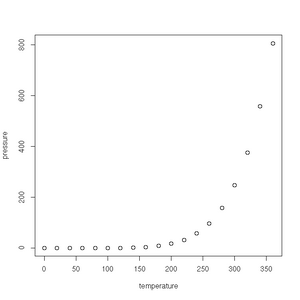
Vapour pressure of mercury against temperature
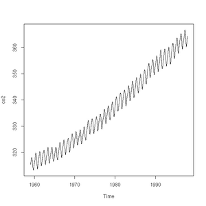
CO2 concentrations measured at Mauna-Loa between 1959 and 1997


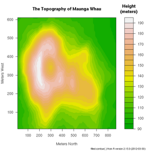
Topology of Maunga Whau volcano in Auckland

Examples of Common Tasks
Linear Regression
> plot(cars)
> res=lm(dist ~ speed, data=cars)
> abline(res)-abline.png)
Exercise
- Weighted least squares. The lm function will accept a vector of weights, lm(... weights=...). If given, the function will optimise the line of best fit according a the equation of weighted least squares. Experiment with different linear model fits, given different weighting vectors. Some handy hints for creating a vector of weights:
- w1<-rep(0.1,50) will give you a vector, length 50, where each element has a value of 0.1. W1[1]<-10 will give the first element of the vector a value of 10.
- w2<-seq(from=0.02, to=1.0, by=0.02) provides a vector containing a sequence of values from 0.02 to 1.0 in steps of 0.02 (handily, again 50 in total).
Significance Testing
> boys_2=c(90.2, 91.4, 86.4, 87.6, 86.7, 88.1, 82.2, 83.8, 91, 87.4)
> girls_2=c(83.8, 86.2, 85.1, 88.6, 83, 88.9, 89.7, 81.3, 88.7, 88.4)
> res=var.test(boys_2,girls_2)
> res=t.test(boys_2, girls_2, var.equal=TRUE, paired=FALSE)