Python1
Python for Scientists
Introduction
With thanks to Simon Metson and Mike Wallace for much of the following material.
Getting Started on BlueCrystal Phase-2
After you have logged in, type the following at the command line:
module add languages/python-2.7.2.0
python
This should start up an interactive python session:
Python 2.7.2 (default, Aug 25 2011, 10:51:03)
[GCC 4.3.3] on linux2
Type "help", "copyright", "credits" or "license" for more information.
>>>
where we can type commands at the >>> prompt.
Python as a Calculator
To get started, let's just try a few commands out. If you type:
>>> print "Hello!"
you'll get:
Hello!
If you try:
>>> print 5 + 9
you'll get:
14
So far so simple! Here is a copy of a session containing a few more commands where we've set the values of some variables and also defined and run our own function:
>>> five = 5
>>> neuf = 9
>>> print five + neuf
14
>>> def say_hello():
...     print "Hello, world!"
... # hit return here
>>> say_hello()
Hello, world!
You can exit an interactive session at any time by typing Ctrl-D.
Getting Help
Python has lots of useful documentation. For example, take a look at: http://docs.python.org/. You can also type help() and the interpreter prompt:
>>> help()

Welcome to Python 2.7!  This is the online help utility.

If this is your first time using Python, you should definitely check out
the tutorial on the Internet at http://docs.python.org/tutorial/.

Enter the name of any module, keyword, or topic to get help on writing
Python programs and using Python modules.  To quit this help utility and
return to the interpreter, just type "quit".

...

help> keywords

Here is a list of the Python keywords.  Enter any keyword to get more help.

and                 elif                if                  print
...

help> if
The ``if`` statement
********************

The ``if`` statement is used for conditional execution:

   if_stmt ::= "if" expression ":" suite
               ( "elif" expression ":" suite )*
               ["else" ":" suite]

It selects exactly one of the suites by evaluating the expressions one
by one until one is found to be true...
...

help> quit

You are now leaving help and returning to the Python interpreter.
...
>>>
Making a Script
An interactive session can be fun and useful for trying things out. However--to save our fingers--we will typically want to execute a series of commands as a script, created using your favourite text editor. Here is the contents of an example script:
#!/bin/env python

print "Hello, from a python script!"
Ensure that your script is executable:
chmod u+x myscript.py
and now you can run it:
[ggdagw@bigblue4 ~]$ ./myscript.py
Hello, from a python script!
Python and Whitespace
Love it of hate it, Python incorporates whitespace in it's syntax. (It's either that or demarcate blocks with some other syntax, such as ending a line with a semi-colon as it is in C. Pick your poison.) Spacing is therefore key in creating a valid python script. For example:
message = "happy days!"
if len(message) > 10:
    print "longer.."
else:
    print "shorter.."
will work, but:
message = "happy days!"
if len(message) > 10:
 print "longer.."
else:
print "shorter.."
will not:
  File "./myscript.py", line 7
    print "shorter.."
        ^
IndentationError: expected an indented block
Nuts and Bolts
Types
Python has intrinsic types including, integers, floats, booleans and complex numbers. It is dynamically typed (meaning that you don't have to have a block of variable declarations at the top of your script), but it is not weakly typed:
>>> my_complex = 2 + 0.5j
>>> my_complex
(2+0.5j)
>>> my_complex.real
2.0
>>> my_complex.imag
0.5
>>> name = 'fred'
>>> lucky = 7
>>> name + lucky
Traceback (most recent call last):
  File "<stdin>", line 1, in <module>
TypeError: cannot concatenate 'str' and 'int' objects
Strings
The eagle-eyed will have spotted in a previous examples that we could ask the length a character string--straight off the bat. No need to write a counting routine ourselves:
print len(message)
We also take slices of our character string. In my case
print message[:5]
Since a string is an object (in the object oriented programming sense of the word, but more of that later...) we can call a number of methods that operate on a string. A selected sample include:
| s.find(sub)) | Finds the first occurrence of the given substring |
| s.islower() | Checks whether all characters are lowercase |
| s.upper() | Returns s converted to uppercase |
| s.strip | Removes leading and trailing whitespace |
| s.replace(old,new) | Replaces substring old with new |
| s.split([sep]) | Splits s uses (optional) sep as a delimiter. Returns a list |
Lists and Tuples
An example of a list is:
shopping = ['bread', 'marmalade', 'milk', 'tea']
and we can inquire about the length of that using the same function as before:
len(shopping)
We can also take slices of a list, as we did with a string:
shopping[0:2]
and even reset a portion of the list that way:
shopping[0:2] = ['bagels', 'jam']
Since a list is also an object, we have more handy methods, including:
| s.append(x) | Appends an new element x to the end of s |
| s.count(x) | Appends an new element x to the end of s |
| s.reverse(x) | Reverses items of s in place |
| s.sort([compfunc]) | Sorts items of s in place. compfunc is an optional comparison function |
Tuples are very similar to lists and support many of the same operations (indexing, slicing, concatenation etc.) but differ in that they are not mutable after creation:
>>> mytuple = ('fred', 'ginger', 7, 2.5)
>>> mylist = ['fred', 'ginger', 7, 2.5]
>>> mylist[2] = 8
>>> print mylist
['fred', 'ginger', 8, 2.5]
>>> print mytuple[2]
7
>>> mytuple[2] = 8
Traceback (most recent call last):
  File "<stdin>", line 1, in <module>
TypeError: 'tuple' object does not support item assignment
List comprehension:
>>> numbers = [12, 3, 90, 40, 52, 11, 10]
>>> small_numbers_doubled = [number * 2 for number in numbers if number < 20]
>>> small_numbers_doubled
[24, 6, 22, 20]
Dictionaries
A dictionary is an associative array or hash table, containing key-value pairs:
mydict = {'thomas':'blue', 'james':'red', 'henry':'green'}
>>> print mydict['james']
red
| m.keys() | Returns a list of the keys in m |
| m.items() | Returns a list of the (key,value) pairs in m |
| m[k] = x | Sets m[k] to x |
| m.update(b) | Adds objects from dictionary b to m |
Control Structures
Here is an if-then-else, python style:
if sky == ‘blue’:
    birds.sing()
elif sky == ‘black’:
    birds.sleep()
else:
    pass #do nothing
and a classic for loop:
for ii in range(1,10):
    print ii
We'll also see a while loop shoehorned into the next example.
For our control statements, we can use comparison operators such as, ==, !=, >, <, <=, >=, and logical operators, such as, and, or,not
File Input and Output
Here's some code for printing the contents of a text file:
fp = open("foo.txt","r")
line = fp.readline()
while line:
    line = line.strip()
    print line
    line.fp.readline()
fp.close()
We could open a file for writing with:
fp = open("foo.txt","w")
Numpy
K, we could spend quite a while getting to grips with all of Python's myriad features, but we'll move onto looking at numerical features and arrays in particular. To do this we will load a package. You can do this by typing:
from numpy import *
Now that we have access to the package, let's create an array. Note that a numpy array is an objects of a different type to an intrinsic array in Python. A simple approach is to use the array function. For example we might enter:
a = array([[1.0,0.0,0.0],[0.0,1.0,0.0],[0.0,0.0,1.0]])
b = array([[1,2,3],[4,5,6],[7,8,9]])
>>> a
array([[ 1.,  0.,  0.],
       [ 0.,  1.,  0.],
       [ 0.,  0.,  1.]])
>>> b
array([[1, 2, 3],
       [4, 5, 6],
       [7, 8, 9]])
>>> transpose(b)
array([[1, 4, 7],
       [2, 5, 8],
       [3, 6, 9]])
Given an array, we may inquire about it's shape:
print a.shape
and we are told that it is a 2-dimensional array (i.e. an array of rank 2) and that the length of both dimensions is 3:
(3, 3)
We can also apply operators to array objects. For example:
a = a * 9
array([[ 9.,  0.,  0.],
       [ 0.,  9.,  0.],
       [ 0.,  0.,  9.]])
Note, however, that most operations on numpy arrays are done element-wise, which may be different to a linear algera operation that you were expecting. We will return to linear algebra operations in a later section.
Should we so desire, we could re-shape the array. One way to do this is to to set it's shape attribute directly:
>>> a.shape = (1,9)
As with the list example, it can be useful to read or change the value of an element (or sub array) indidually. Let's turn the array back to it's rank-2 form and try it out:
>>> a.shape = (3,3)
>>> a[1,1] = 777.0
>>> print a
>>> a[1:,1:] = [[777.0, 777.0],[777.0, 777.0]]
>>> print a
This is all pretty handy so far, but specifying the value of each element explicitly could become a chore. Happily some helper functions exist to give you a head start with some building blocks. For example, your can use:
>>> b = zeros((3,3)
>>> print b
>>> b = ones((3,2))
>>> print b
>>> b = identity(2)
>>> print b
>>> big = resize(b, (6,6))
>>> print big
The use of resize in the last example illustrates a useful replicating feature.
A list of all the functions and operations contained within numpy is: http://scipy.org/Numpy_Example_List.
Pylab and Matplotlib
The above examples are quite natty, but we have deliberately kept the array sizes small so that we can print the element values easily. In practice, you may find that your array sizes are much larger and printing the values to the screen is impractical. Fear not! Python has many packages which help you plot your data, so that you can explore it.
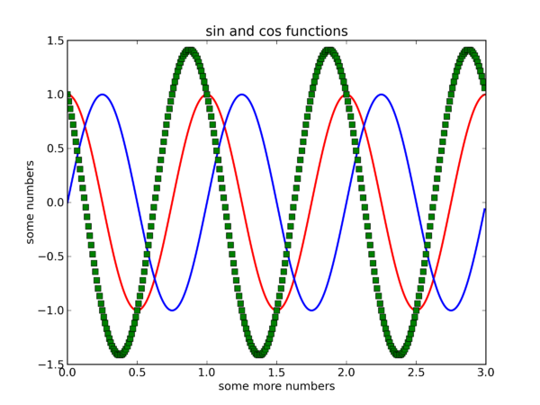
Using the pylab plotting interface we can create:
import pylab
from numpy import arange, pi, cos, sin
t = arange(0.0, 3.0, 0.01)
c = cos(2 * pi * t)
s = sin(2 * pi * t)
pylab.ylabel('some numbers')
pylab.xlabel('some more numbers')
pylab.plot(t, c, 'r', lw=2)
pylab.plot(t, s, 'b', lw=2)
pylab.plot(t, c-s, 'gs', lw=2)
pylab.ylim(-1.5, 1.5)
pylab.title('sin and cos functions')
pylab.savefig('curves', dpi=300)
Where curves.png looks like:
You can open .png images from the linux command line (inc. bluecrystal) using, e.g.: display -resize 1000 curves.png
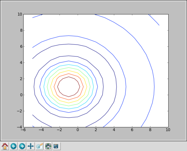
We can also use Matplotlib directly for more control:
>>> x = arange(-5,10)
>>> y = arange(-4,11)
>>> z1 = sqrt(add.outer(x**2,y**2))
>>> Z = sin(z1)/z1
>>> import matplotlib.pyplot as plt
>>> from pylab import meshgrid
>>> X, Y = meshgrid(x,y)
>>> plt.figure()
>>> plt.contour(X,Y,Z)
>>> plt.show()
and you should get a window similar to:
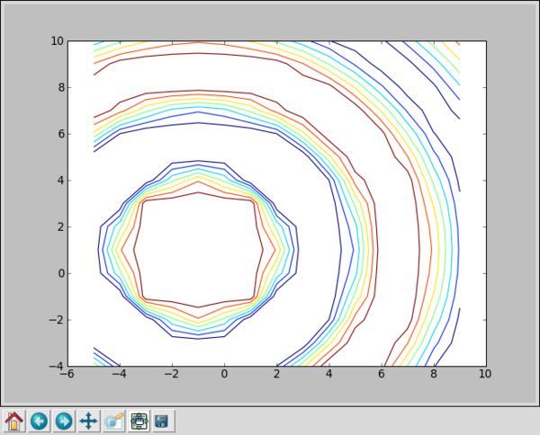
The clip function is an interesting one. Using it, we can replace values greater than some threshold with a ceiling and lower than another threshold with a floor. For example:
>>> Z1 = clip(Z,-0.1,0.1)
>>> plt.figure()
>>> plt.contour(X,Y,Z1)
>>> plt.show()
gives us:
Input and Output
The foregoing is all very interesting, but life would be rather dull if you had to re-enter all your data by hand whenever you set to work with Python and numpy. Therefore we need a means to save data to a file and load it again. Happily, we can do this rather easily using a couple of routines from the pylab package:
>>> from numpy import *
>>> from pylab import load
>>> from pylab import save
>>> data = zeros((3,3))
>>> save('myfile.txt', data)
>>> read_data = load("myfile.txt")
warning, the load() function of numpy will be shadowed in the above example. One way to protect yourself against this is to make use of namespaces: Modify your import command to import pylab and then use pylab.load(..).
Scipy
- http://www.scipy.org/
- ..and good examples on http://scipy-lectures.github.com/intro/scipy.html
- Many useful features:
- Integration
- Optimisation (curve fitting, etc)
- Fourier transforms
- Signal processing
- Statistical algorithms
- Much, much more...
- If you know Python you can use SciPy


