Difference between revisions of "NumMethodsPDEs"
| Line 217: | Line 217: | ||
---- | ---- | ||
| − | [[LinAlgebraPacks]] contains an exercise in which you see what happens if the CFL condition is not satisfied. | + | '''Exercise''' |
| + | |||
| + | * [[LinAlgebraPacks]] contains an exercise in which you see what happens if the CFL condition is not satisfied. | ||
==Parabolic Equations: Backward (Implicit) Euler== | ==Parabolic Equations: Backward (Implicit) Euler== | ||
Revision as of 14:22, 11 July 2011
Numerical Methods for PDEs: Solving PDEs on a computer
Introduction
In this tutorial we're going to look at how to solve Partial Differential Equations (PDEs) numerically. That is, on a computer, as opposed to analytically, as we may be able to do so with our brains and a pencil and paper. PDEs crop up a good deal when we come to try and describe things in the world--such as the flow of heat, or the distribution of electrical charge--and so methods for their solution prove to be handy over and over again when we want to model the natural world.
At the outset, let's list some of the take-home messages from the material below:
- Finding a numerical solution to a PDE often boils down to solving a system of linear equations, of the (matrix) form Ax=b.
- Third party linear algebra libraries will be much faster and less error prone than your own code for this task. Many of these libraries will also execute in a parallel fashion.
- The matrix A is often sparse and so iterative methods will often be much faster than performing a direct method for solution (such as an LU decomposition).
Looking at Nature (& a quick philosophical aside)
When we observe nature, certain patterns crop up again and again. For example, in the the field of electrostatics, if a function [math]\displaystyle{ f }[/math] describes a distribution of electric charge, then Poisson's equation:
- [math]\displaystyle{ {\nabla}^2 u = f. }[/math]
gives the electric potential [math]\displaystyle{ u }[/math].
However, Poisson's equation also describes the steady state temperature of a material when subjected to some heating and also crops up when considering gravitational potentials..
What's going on here? Why are we using the same equation? Is Poisson's equation fundamental in some way? Well, yes I suppose it is. However, we can look at it another way and say that Poisson's equation is the way we describe--using the language of maths--steady state phenomena which involve potentials. OK, this sounds a bit out there, but consider the following very general equation for a moment (it's a second-order linear equation in two variables):
[math]\displaystyle{ Au_{xx} + Bu_{xy} + Cu_{yy} + Du_x + Eu_y + Fu = G }[/math]
It turns out that we can categorise certain instances of this equation and then relate these categories to the kind of phenomena that they describe:
- Parabolic: [math]\displaystyle{ B^2 - 4AC = 0 }[/math]. This family of equations describe heat flow and diffusion processes.
- Hyperbolic: [math]\displaystyle{ B^2 - 4AC \gt 0 }[/math]. Describe vibrating systems and wave motion.
- Elliptic: [math]\displaystyle{ B^2 - 4AC \lt 0 }[/math]. Steady-state phenomena.
That's pretty handy! OK, we've had our philosophical aside, on with the show.
The Finite Difference Method
In this section we'll look at solving PDEs using the Finite Difference Method. Finite difference equations have a long and illustrious past. Indeed, they were used by Newton-and-the-gang as a logical route in to talk about differential calculus. So, in fact, we're just going to work back in the other direction..
Discritisation
The functions and variables that we see in, for instance, Poisson's equation are continuous; meaning that they could have an infinite number of values. This is fine when solving equations analytically, but we are limited to considering only a finite number of values when solving PDEs using a digital computer. We need a way to discritise our problems. Happily, help is at hand from the (sometimes tortuous) Taylor series: We can approximate the value of a function at a point distant from x (i.e. displaced by an amount h) using a linear summation of derivatives of the function at x--a Taylor expansion:
- [math]\displaystyle{ f(x+h) \approx f(x) + \frac{f'(x)}{1!}h + \frac{f''(x)}{2!}h^2 + \cdots }[/math]
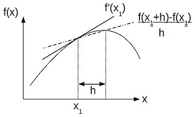
We can truncate this series after the first differential and rearrange, to get ourselves the forward-difference approximation:
- [math]\displaystyle{ f'(x) \approx \frac{f(x+h) - f(x)}{h} }[/math]
Thus, following the finite difference approach, we can discritise our equations by replacing our differential operators by their difference approximations, as helpfully provided by a truncated Taylor series. If, like me, you like thinking visually, the schematic below shows the relationship between a differential operator--the gradient at a point [math]\displaystyle{ x_1 }[/math] and the finite difference approximation to the gradient:
If we were to consider a displacement of -h instead, we would get the backward-difference approximation to [math]\displaystyle{ f'(x) }[/math]:
- [math]\displaystyle{ f'(x) \approx \frac{f(x) - f(x-h)}{h} }[/math],
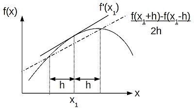
Subtracting the backward difference from the forward difference we get the central-difference approximation:
- [math]\displaystyle{ f'(x) \approx \frac{1}{2h}(f(x+h) - f(x-h)) }[/math].
By retaining an extra term from the Taylor series, and some similar rearrangements, we can also formulate a finite difference approximation to the 2nd differential. For example the central-difference formula for this is:
- [math]\displaystyle{ f''(x) \approx \frac{1}{h^2} [ f(x+h) - 2f(x) + f(x-h) ] }[/math].
In a similar way we can derive formulae for approximations to partial derivatives. Armed with all these formulae, we can convert differential equations into difference equations, which we can solve on a computer. However, since we are dealing with approximations to the original equation(s), we must be vigilant that errors in our input and intermediate calculations do not accumulate such that our final solution is meaningless.
Eliptical Equations: Discrete Laplacian Operator
Now that we have our difference formulae, let's apply them to Laplace's equation in 2-dimensions:
- [math]\displaystyle{ \frac{\partial^2u}{\partial x^2} + \frac{\partial^2u}{\partial y^2} = 0 }[/math]
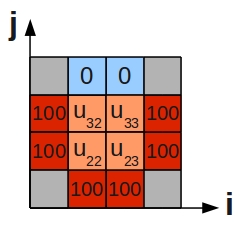
This describes purely diffusive phenomena and can give us, for example, the steady state temperature over a 2D plate. Let's suppose that three sides of the plate are held at 100°C, while the fourth is held at 0°C. We can divide the plate into a number of grid cells:
Using the central difference approximation to a 2nd differential that we derived in the last section, we can rewrite the differential equation as a difference equation:
- [math]\displaystyle{ \frac{\partial^2u}{\partial x^2} + \frac{\partial^2u}{\partial y^2} \approx \frac{1}{h^2}(u^j_{i+1} -2u^j_i +u^j_{i-1}) + \frac{1}{k^2}(u^{j+1}_i -2u^j_i +u^{j-1}_i) }[/math]
where h is the grid spacing in the i-directions and k is the spacing the j-direction. If we set [math]\displaystyle{ h=k }[/math], then:
- [math]\displaystyle{ u^j_{i+1} + u^j_{i-1} + u^{j+1}_i + u^{j-1}_i - 4u^j_i = 0 }[/math]
solving for [math]\displaystyle{ u^j_i }[/math]:
- [math]\displaystyle{ u^j_i = \frac{1}{4}(u^j_{i+1} + u^j_{i-1} + u^{j+1}_i + u^{j-1}_i) }[/math]
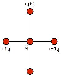
Note that this last equation says--quite intuitively--that the value at the central grid point is equal to the average of its four neighbours. We can draw a picture of the stencil needed to compute the central value:
Centring the stencil on each of the 4 grid cells of the inner region (orange) in turn, we generate the following 4 difference equations:
- [math]\displaystyle{ \begin{alignat}{5} -4u_{22} & + u_{32} & + u_{23} & + 100 & + 100 & = 0 \\ -4u_{32} & + 0 & + u_{33} & + u_{22} & + 100 & = 0 \\ -4u_{23} & + u_{33} & + 100 & + 100 & + u_{22} & = 0 \\ -4u_{33} & + 0 & + 100 & + u_{23} & + u_{32} & = 0 \\ \end{alignat} }[/math]
This system of equations can be written in matrix form:
- [math]\displaystyle{ \begin{bmatrix}-4 & 1 & 1 & 0\\1 & -4 & 0 & 1\\1 & 0 & -4 & 1\\0 & 1 & 1 & -4\end{bmatrix} \begin{bmatrix}u_{22}\\u_{32}\\u_{23}\\u_{33}\end{bmatrix} = \begin{bmatrix}-200\\-100\\-200\\-100\end{bmatrix} }[/math]
Which may be summarised as the vector equation, Ax=b, which can be efficiently & conveniently solved using a library linear algebra routines, such as LAPACK, PETSc or PLASMA.
Parabolic Equations: Forward (Explicit) Euler
Let's look at how to solve a different class of equation, again using finite difference techniques.
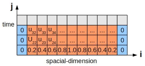
An example of a parabolic equation is the 1D heat equation, which describes the evolution of temperature at various points in a thin, insulated bar over time. Imagine such a bar where the ends are kept at 0°C:
Since this scenario involves the passage of time, just stating the boundary conditions is not enough, and we must also specify some initial condition for the temperature along the bar's length. This is shown below for a bar divided up into grid cells, as before:
The 1D heat equation is:
- [math]\displaystyle{ \frac{\partial u}{\partial t}=\alpha \frac{\partial^2u}{\partial x^2} }[/math]
where [math]\displaystyle{ \alpha }[/math]--the thermal diffusivity--is set to 1 for simplicity. One way to rewrite this as a difference equation (using a forward difference for the LHS and a central difference for the RHS*) is:
- [math]\displaystyle{ \frac{u^{j+1}_i - u^j_i }{k} = \frac{u^j_{i+1} - 2u^j_i + u^j_{i-1}}{h^2} }[/math]
and rearrange to solve for [math]\displaystyle{ u^{j+1}_i }[/math]:
- [math]\displaystyle{ u^{j+1}_i = u^j_i + r(u^j_{i+1} - 2u^j_i + u^j_{i-1}) }[/math]
- [math]\displaystyle{ u^{j+1}_i = ru^j_{i+1} + (1- 2r)u^j_i + ru^j_{i-1} }[/math]
where:
[math]\displaystyle{ r=\frac{k}{h^2} }[/math]
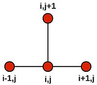
This time, we see that the appropriate stencil is:
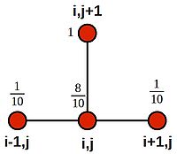
If we set [math]\displaystyle{ h=\frac{1}{10} }[/math] and [math]\displaystyle{ k=\frac{1}{1000} }[/math], then [math]\displaystyle{ r=\frac{1}{10} }[/math], and the equation becomes:
- [math]\displaystyle{ u^{j+1}_i = u^j_i + \frac{1}{10}(u^j_{i+1} - 2u^j_i + u^j_{i-1}) }[/math]
- [math]\displaystyle{ u^{j+1}_i = \frac{1}{10}(u^j_{i+1} + 10u^j_i - 2u^j_i + u^j_{i-1}) }[/math]
- [math]\displaystyle{ u^{j+1}_i = \frac{1}{10}(u^j_{i+1} + 8u^j_i + u^j_{i-1}) }[/math]
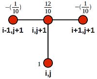
Which we can illustrate using weightings on the stencil nodes:
Forward Euler is as an explicit method, as one unknown value ([math]\displaystyle{ u^{j+1}_i }[/math]) is expressed directly in terms of known values (all values of u at time j are known).
We could implement a simple marching algorithm, where we centre the stencil over a set of known values at time j, and may calculate the unknown temperature for grid cell i at time j+1. However, it would be better to group together all the calculations for a particular time step into a system of simultaneous equations (for our example 1d heat problem):
- [math]\displaystyle{ u_{22} = \frac{1}{10}(0) + \frac{8}{10}(0.2) + \frac{1}{10}(0.4) }[/math]
- [math]\displaystyle{ u_{23} = \frac{1}{10}(0.2) + \frac{8}{10}(0.4) + \frac{1}{10}(0.6) }[/math]
- [math]\displaystyle{ u_{24} = \frac{1}{10}(0.4) + \frac{8}{10}(0.6) + \frac{1}{10}(0.8) }[/math]
- [math]\displaystyle{ \cdots }[/math]
and then re-write in matrix form:
- [math]\displaystyle{ \begin{bmatrix}u_{22} \\ u_{23} \\ u_{24} \\\vdots \end{bmatrix} = \begin{bmatrix} 0.1 & 0.8 & 0.1 & 0 & 0 & \cdots & 0 \\ 0 & 0.1 & 0.8 & 0.1 & 0 & \cdots & 0 \\ \vdots & & & & & & \vdots \\ & & \cdots & 0 & 0.1 & 0.8 & 0.1 \\ \end{bmatrix} \times \begin{bmatrix}0 \\ 0.2 \\ 0.4 \\ \vdots \\ 0.2 \\ 0 \end{bmatrix} }[/math]
as the computational efficiency of a matrix vector multiplication will be hard to better. Note that we can write the above piece of linear algebra in a general form:
- [math]\displaystyle{ \begin{bmatrix}u_{22} \\ u_{23} \\ u_{24} \\ \vdots \end{bmatrix} = \begin{bmatrix} r & 1-2r & r & 0 & 0 & \cdots & 0 \\ 0 & r & 1-2r & r & 0 & \cdots & 0 \\ \vdots & & & & & & \vdots \\ & & \cdots & 0 & r & 1-2r & r \\ \end{bmatrix} \times \begin{bmatrix}u_{11} \\ u_{12} \\ u_{13} \\ u_{14} \\ \vdots \end{bmatrix} }[/math]
(*The two difference schemes for either side of the equation were chosen so that the approximation error characteristics for either side are approximately balanced and so the errors on one side or the other do not begin to dominate the calculations.)
Solution Stability and the CFL Condition
The Forward Euler scheme has the benefit of simplicity, but is unstable for large time steps. The CFL (Courant–Friedrichs–Lewy) condition states that the following must hold:
- [math]\displaystyle{ r=\frac{k}{h^2} \le 0.5 }[/math]
for stability.
Exercise
- LinAlgebraPacks contains an exercise in which you see what happens if the CFL condition is not satisfied.
Parabolic Equations: Backward (Implicit) Euler
Another way to formulate our finite difference equations for the very same problem is to use backward-differences instead of forward-differences. The backward Euler scheme requires more computation per time-step than the forward scheme, but has the distinct advantage that it is unconditionally stable with regard to the relative size between the time and spatial step sizes; i.e. we are not limited to [math]\displaystyle{ r \le 0.5 }[/math] when we use the backward Euler scheme.
We will use a central-difference on the RHS, as before, but shifting the time index to [math]\displaystyle{ j+1 }[/math]. This will allow us to formulate a backward-difference on the RHS between the time indices [math]\displaystyle{ j }[/math] and [math]\displaystyle{ j+1 }[/math]:
- [math]\displaystyle{ \frac{u^{j+1}_i - u^j_i }{k} = \frac{u^{j+1}_{i+1} - 2u^{j+1}_i + u^{j+1}_{i-1}}{h^2} }[/math]
- [math]\displaystyle{ u^{j+1}_i - u^j_i = \frac{k}{h^2}(u^{j+1}_{i+1} - 2u^{j+1}_i + u^{j+1}_{i-1}) }[/math]
- [math]\displaystyle{ u^{j+1}_i - u^j_i = r(u^{j+1}_{i+1} - 2u^{j+1}_i + u^{j+1}_{i-1}) }[/math]
- [math]\displaystyle{ u^{j+1}_i - u^j_i = ru^{j+1}_{i+1} - 2ru^{j+1}_i + ru^{j+1}_{i-1} }[/math]
- [math]\displaystyle{ u^{j+1}_i - ru^{j+1}_{i+1} + 2ru^{j+1}_i - ru^{j+1}_{i-1} = u^j_i }[/math]
- [math]\displaystyle{ u^j_i = - ru^{j+1}_{i+1} + (1 + 2r)u^{j+1}_i - ru^{j+1}_{i-1} }[/math]
If we again choose [math]\displaystyle{ h=\frac{1}{10} }[/math] and [math]\displaystyle{ k=\frac{1}{1000} }[/math], such that [math]\displaystyle{ r=\frac{k}{h^2}=\frac{1}{10} }[/math], as before, we end up with the following system of equations when we consider all values of [math]\displaystyle{ i }[/math] for our first time-step--from [math]\displaystyle{ j }[/math] to [math]\displaystyle{ j+1 }[/math]--where we know values of all the cells at time [math]\displaystyle{ j }[/math]:
- [math]\displaystyle{ 0.2 = -\frac{1}{10}(0) + \frac{12}{10}(u_{22}) -\frac{1}{10}(u_{23}) }[/math]
- [math]\displaystyle{ 0.4 = -\frac{1}{10}(u_{22}) + \frac{12}{10}(u_{23}) -\frac{1}{10}(u_{24}) }[/math]
- [math]\displaystyle{ 0.6 = -\frac{1}{10}(u_{23}) + \frac{12}{10}(u_{24}) -\frac{1}{10}(u_{25}) }[/math]
- [math]\displaystyle{ \cdots }[/math]
We can see that this is akin to looping over the domain with the following stencil:
Rearranging, so that we have only constants on the RHS:
- [math]\displaystyle{ \frac{1}{10}(0) + \frac{12}{10}(u_{22}) -\frac{1}{10}(u_{23}) = 0.2 + \frac{1}{10}(0) }[/math]
- [math]\displaystyle{ \frac{1}{10}(u_{22}) + \frac{12}{10}(u_{23}) -\frac{1}{10}(u_{24}) = 0.4 }[/math]
- [math]\displaystyle{ \frac{1}{10}(u_{23}) + \frac{12}{10}(u_{24}) -\frac{1}{10}(u_{25}) = 0.6 }[/math]
- [math]\displaystyle{ \cdots }[/math]
We can re-write this system of equations in matrix form:
- [math]\displaystyle{ \begin{bmatrix} 1.2 & -0.1 & 0 & 0 & \cdots & 0 \\ -0.1 & 1.2 & -0.1 & 0 & \cdots & 0 \\ \vdots & & & & & \vdots \\ & & \cdots & 0 & -0.1 & 1.2 \\ \end{bmatrix} \times \begin{bmatrix} u_{22} \\ u_{23} \\ u_{24} \\\vdots \end{bmatrix} = \begin{bmatrix} 0.2 + 0.1(0) \\ 0.4 \\ \vdots \\ 0.2 +0.1(0) \end{bmatrix} }[/math]
The general form is:
- [math]\displaystyle{ \begin{bmatrix} 1+2r & -r & 0 & 0 & \cdots & 0 \\ -r & 1+2r & -r & 0 & \cdots & 0 \\ \vdots & & & & & \vdots \\ & & \cdots & 0 & -r & 1+2r \\ \end{bmatrix} \times \begin{bmatrix} u_{22} \\ u_{23} \\ u_{24} \\\vdots \end{bmatrix} = \begin{bmatrix} u_{12} + r(u_{11}) \\ u_{13} \\ \vdots \\ u_{1n-1} + r(u_{1n}) \end{bmatrix} }[/math]
Parabolic Equations: Crank-Nicolson
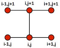
Now, forward and backward Euler schemes are by far from the only ways in which to approach this 1D heat problem. Yet another scheme is the to create finite difference equations using the Crank-Nicolson stencil:
The stencil amounts to an average of both the forward and backward Euler methods. The resulting difference equation is:
- [math]\displaystyle{ \frac{u^{j+1}_i - u^j_i}{k} = \frac{1}{2}(\frac{u^{j+1}_{i+1} - 2u^{j+1}_{i} + u^{j+1}_{i-1}}{h^2} + \frac{u^j_{i+1} - 2u^j_i + u^j_{i-1}}{h^2}). }[/math]
Which we may rearrange to become:
- [math]\displaystyle{ u^{j+1}_i - u^j_i = \frac{1}{2}\frac{k}{h^2}(u^{j+1}_{i+1} - 2u^{j+1}_i + u^{j+1}_{i-1} + u^j_{i+1} - 2u^j_i + u^j_{i-1}) }[/math]
- [math]\displaystyle{ 2(u^{j+1}_i - u^j_i) = r(u^{j+1}_{i+1} - 2u^{j+1}_i + u^{j+1}_{i-1} + u^j_{i+1} - 2u^j_i + u^j_{i-1}) }[/math],
where [math]\displaystyle{ r=\frac{k}{h^2} }[/math].
Collecting the unknowns (values of u at the next timestep, [math]\displaystyle{ j+1 }[/math]) to the LHS and the knowns (values of u at current timestep, [math]\displaystyle{ j }[/math]), we get:
- [math]\displaystyle{ 2u^{j+1}_i + 2ru^{j+1}_i - ru^{j+1}_{i+1} - ru^{j+1}_{i-1} = 2u^j_i +ru^j_{i+1} -2ru^j_i + ru^j_{i-1} }[/math]
- [math]\displaystyle{ (2+2r)u^{j+1}_i - ru^{j+1}_{i+1} - ru^{j+1}_{i-1} = (2-2r)u^j_i +ru^j_{i+1} + ru^j_{i-1} }[/math].
If we choose [math]\displaystyle{ h=1/10 }[/math] and [math]\displaystyle{ k=1/100 }[/math] (note that the time-step is 10x larger than than chosen for the forward Euler example), then [math]\displaystyle{ r=1 }[/math], and we get:
- [math]\displaystyle{ -u_{i-1}^{j+1} +4u_i^{j+1} -u_{i+1}^{j+1} = u_{i-1}^j + u_{i+1}^j }[/math].
We can again create a system of linear equations for all the cells j along the bar at a given time step i:
- [math]\displaystyle{ -0 + 4u_{22} - u_{23} = 0 + 0.4 }[/math]
- [math]\displaystyle{ -u_{22} + 4u_{23} - u_{24} = 0.2 + 0.6 }[/math]
- [math]\displaystyle{ -u_{23} + 4u_{24} - u_{25} = 0.4 + 0.8 }[/math]
- [math]\displaystyle{ \cdots }[/math]
We have [math]\displaystyle{ j }[/math] unknowns and [math]\displaystyle{ j }[/math] equations. Then we can again translate into matrix notation and solve using a library linear algebra routines:
- [math]\displaystyle{ \begin{bmatrix} -4 & 1 & 0 & 1 & 0 & 0 & \cdots & 0 \\ 1 & -4 & 1 & 0 & 1 & 0 & \cdots & 0 \\ \vdots & & & & & & & \vdots \\ & \cdots & & 0 & 1 & 0 & 1 & -4\\ \end{bmatrix} \times \begin{bmatrix} u_{22} \\ u_{23} \\ u_{24} \\\vdots \end{bmatrix} = \begin{bmatrix} 0 + 0.4 \\ 0.2 + 0.6 \\ \vdots \\ 0 + 0.4 \end{bmatrix} }[/math]
In general:
- [math]\displaystyle{ \begin{bmatrix} -(2+2r) & r & 0 & r & 0 & 0 & \cdots & 0 \\ r & -(2+2r) & r & 0 & r & 0 & \cdots & 0 \\ \vdots & & & & & & & \vdots \\ & \cdots & & 0 & r & 0 & r & -(2+2r)\\ \end{bmatrix} \times \begin{bmatrix} u_{22} \\ u_{23} \\ u_{24} \\\vdots \end{bmatrix} = \begin{bmatrix} ru_{11} + (2-2r)u_{12} + ru_{13} \\ \vdots \end{bmatrix} }[/math]
Other Numerical Methods
We have looked at the finite difference method (FDM) above, but other (more mathsy) approaches exist, such as the finite element and finite volume methods. Each approach has its pros and cons. For example, the FDM is limited to regular grids spread over rectangular domains, but is easy to program. In contrast the FEM is applicable to intricately shaped domains and the resolution of the individual elements can be varied, but is requires more involved programming and a deeper level of understand of the relevant mathematics. It should also be noted, however, that under certain circumstances, the FEM and FVM boil down to be exactly the same as the FDM, even though we've approached the task of solving a PDE from a different direction.
One thing which is always common to the approaches is that the problem boils down to a system of linear equations to solve, and that a library of linear algebra routines will be the workhorse when finding solutions to PDEs on a computer. Repeat after me, "a fast linear algebra library is key!"
The Finite Element Method (FEM)
The general approach here is to create a potential function from our PDE and to find a solution to it via minimising the potential function. Key steps include:
- Discritisation of the original PDE, often by proposing that we can approximate the solution using a linear sum of (polynomial) basis functions.
- Create the potential function by invoking the method of weighted residuals, and in particular the Galerkin specialisation of this approach.
- Use whatever algebraic manipulation and integration (possibly numerical) is required to create a system of linear equations.
- Solve said system of linear equations and in doing so, solve the original PDE.
For example, consider again Poisson's equation over a 2-dimensional region, [math]\displaystyle{ R }[/math]:
- [math]\displaystyle{ \nabla^2u=f(x,y) }[/math]
where [math]\displaystyle{ u=0 }[/math] at the boundary of the domain.
Next, applying the method of weighted residuals, we multiply both sides by weighting functions [math]\displaystyle{ \phi_i }[/math], and take integrals over the domain:
- [math]\displaystyle{ \iint\limits_R \nabla^2u\phi_i\, dA = \iint\limits_R f\phi_i\, dA }[/math]
We can apply integration-by-parts to the LHS ([math]\displaystyle{ \phi_i\nabla^2u }[/math]), for example:
- [math]\displaystyle{ \int \phi_i\nabla^2 u = \phi_i\nabla u - \int \nabla\phi_i \cdot \nabla u }[/math]
Differentiating both sides:
- [math]\displaystyle{ \phi_i\nabla^2 u = \nabla \cdot (\phi_i\nabla u) - \nabla\phi_i \cdot \nabla u }[/math]
So inserting this into our equation for weighted residuals, above:
- [math]\displaystyle{ \iint\limits_R [\nabla \cdot (\phi_i\nabla u) - \nabla\phi_i \cdot \nabla u]\, dA = \iint\limits_R f\phi_i\, dA }[/math]
and rearranging, we get:
- [math]\displaystyle{ \iint\limits_R \nabla\phi_i \cdot \nabla u\, dA = \iint\limits_R \nabla \cdot (\phi_i\nabla u)\, dA - \iint\limits_R f\phi_i\, dA }[/math]
We can see that the 1st term on the RHS is a divergence(the divergence of a vector field [math]\displaystyle{ F }[/math], [math]\displaystyle{ div F = \nabla \cdot F }[/math]), and so we can apply Gauss' Divergence Theorem which states, for the region [math]\displaystyle{ R }[/math] bounded by the curve s:
- [math]\displaystyle{ \iint\limits_R \nabla \cdot F\, dA = \oint\limits_s F \cdot n\, ds }[/math]
where [math]\displaystyle{ n }[/math] is the unit vector normal to the surface.
and so,
- [math]\displaystyle{ \iint\limits_R \nabla\phi_i \cdot \nabla u\, dA = \oint\limits_s \phi_i\nabla u \cdot n\, ds - \iint\limits_R f\phi_i\, dA }[/math]
but our homogeneous boundary conditions also tell us that [math]\displaystyle{ u }[/math] is equal to zero at the boundary and so the 1st term on the RHS goes to zero:
- [math]\displaystyle{ \iint\limits_R \nabla\phi_i \cdot \nabla u\, dA = - \iint\limits_R f\phi_i\, dA }[/math]
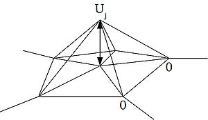
So far, all of the operations above have been done on our unaltered, continuous differential equation. At this point, let's introduce the discritisation--and hence the approximation--that we need to make to work on a digital computer. We intend to approximate the solution [math]\displaystyle{ u(x,y) }[/math] using a linear combination of basis functions:
- [math]\displaystyle{ U(x,y) = \sum_{j=1}^m U_j\phi_j(x,y) }[/math]
The Galerkin method is being used here, as our basis functions are the same as the weighting functions used above.
- [math]\displaystyle{ \sum_{j=1}^m U_j \iint\limits_R \nabla\phi_i \cdot \nabla\phi_j \, dA = - \iint\limits_R f\phi_i\, dA }[/math]
At this point, we can introduce a symmetric 'stiffness matrix' with entries:
- [math]\displaystyle{ K_{ij} = \iint\limits_R \nabla\phi_i \cdot \nabla\phi_j \, dA }[/math]
and a vector F, with entries:
- [math]\displaystyle{ F_i = - \iint\limits_R f\phi_i\, dA }[/math]
and thus our [math]\displaystyle{ m }[/math] equations:
- [math]\displaystyle{ \sum_{j=1}^m K_{ij}U_j = F_i }[/math]
which, we see, yet again is a linear system of equations of the form Ax=b. Cue a call to a linear algebra library!
If we use linear basis functions over our domain, we will end up with the same system of linear equations to solve as we would get following the FDM:
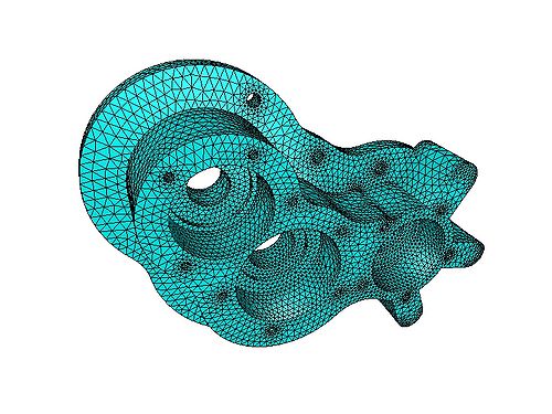
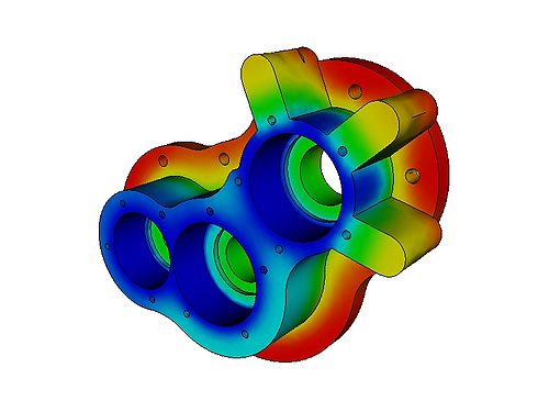
Rather than trying to write an example program to demonstrate the FEM, it makes much more sense to look at a freely available FEM package, such as Elmer (http://www.csc.fi/english/pages/elmer). Below are images obtained by running one of the examples included with Elmer:
