Difference between revisions of "NumMethodsPDEs"
| Line 180: | Line 180: | ||
=Parabolic Equations: Backward Euler= | =Parabolic Equations: Backward Euler= | ||
| − | + | An alternative way to formulate our finite difference is to use a backward difference on the LHS, keeping the central difference on the RHS, but shifting the time index to j+1, so as maintain a backward difference on the LHS: | |
| + | |||
| + | :<math>\frac{u^{j+1}_i - u^j_i }{k} = \frac{u^{j+1}_{i+1} - 2u^{j+1}_i + u^{j+1}_{i-1}}{h^2}</math> | ||
| + | |||
| + | :<math>u^{j+1}_i - u^j_i = \frac{k}{h^2}(u^{j+1}_{i+1} - 2u^{j+1}_i + u^{j+1}_{i-1})</math> | ||
| + | |||
| + | :<math>u^{j+1}_i - u^j_i = r(u^{j+1}_{i+1} - 2u^{j+1}_i + u^{j+1}_{i-1})</math> | ||
| + | |||
| + | :<math>u^{j+1}_i - u^j_i = ru^{j+1}_{i+1} - 2ru^{j+1}_i + ru^{j+1}_{i-1}</math> | ||
| + | |||
| + | :<math>u^{j+1}_i - ru^{j+1}_{i+1} + 2ru^{j+1}_i - ru^{j+1}_{i-1} = u^j_i</math> | ||
| + | |||
| + | :<math>u^j_i = - ru^{j+1}_{i+1} + (1 + 2r)u^{j+1}_i - ru^{j+1}_{i-1}</math> | ||
=Parabolic Equations: Crank-Nicolson= | =Parabolic Equations: Crank-Nicolson= | ||
Revision as of 10:39, 9 April 2011
Numerical Methods for PDEs: Solving PDEs on a computer
Introduction
In this tutorial, we'll take a look at how we might model aspects of the world around us on a computer. When we use mathematics to describe many of the phenomena that we see we end up using Partial Differential Equations (PDEs), and so we seek ways to solve these numerically.
Looking at Nature (& a quick philosophical aside)
When we observe nature, certain patterns crop up again and again. For example, in the the field of electrostatics, if a function [math]\displaystyle{ f }[/math] describes a distribution of electric charge, then Poisson's equation:
- [math]\displaystyle{ {\nabla}^2 \varphi = f. }[/math]
gives the electric potential [math]\displaystyle{ \varphi }[/math].
However, Poisson's equation also describes the steady state temperature of a material when subjected to some heating and also crops up when considering gravitational potentials..
What's going on here? Why the recycling of the same equation? Is Poisson's equation fundamental in some way? Well, yes I suppose it is. However, we can look at it another way and say that Poisson's equation is the way we describe--using the language of maths--steady state phenomena which involve potentials. OK, this sounds a bit out there, but consider the following very general equation for a moment (it's a second-order linear equation in two variables):
[math]\displaystyle{ Au_{xx} + Bu_{xy} + Cu_{yy} + Du_x + Eu_y + Fu = G }[/math]
It turns out that we can categorise certain instances of this equation and then relate these categories to the kind of phenomena that they describe:
- Parabolic: [math]\displaystyle{ B^2 - 4AC = 0 }[/math]. This family of equations describe heat flow and diffusion processes.
- Hyperbolic: [math]\displaystyle{ B^2 - 4AC \gt 0 }[/math]. Describe vibrating systems and wave motion.
- Elliptic: [math]\displaystyle{ B^2 - 4AC \lt 0 }[/math]. Steady-state phenomena.
That's pretty handy!
Discritisation
OK, so far so good. However, the functions and variables that we've considered thus far are continuous, meaning that they could have an infinite number of values. This is fine when solving equations analytically, but we need to deal with a finite number of values when working with a digital computer. We need a way to discritise our problems. Happily, help is at hand from the Taylor series. Recall that we can approximate the value of a function at a point distant (displaced by an amount h) from x using a linear summation of derivatives of the function at x:
- [math]\displaystyle{ f(x+h) \approx f(x) + \frac{f'(x)}{1!}h + \frac{f''(x)}{2!}h^2 + \cdots }[/math]
Let's truncate this series after the first differential and rearrange, to get ourselves the forward-difference approximation:
- [math]\displaystyle{ f'(x) \approx \frac{f(x+h) - f(x)}{h} }[/math]
If we were to consider a displacement of -h instead, we would get the backward-difference approximation to [math]\displaystyle{ f'(x) }[/math]:
- [math]\displaystyle{ f'(x) \approx \frac{f(x) - f(x-h)}{h} }[/math],
Subtracting the backward from the forward we can generate the central-difference approximation:
- [math]\displaystyle{ f'(x) \approx \frac{1}{2h}(f(x+h) - f(x-h)) }[/math].
By retaining an extra term from the Taylor series, and some similar rearrangements, we can also formulate a finite difference approximation to the 2nd differential. For example the central-difference formula for this is:
- [math]\displaystyle{ f''(x) \approx \frac{1}{h^2} [ f(x+h) - 2f(x) + f(x-h) ] }[/math].
In a similar way we can derive formulae for approximations to partial derivatives. Armed with all these formulae, we can convert differential equations into difference equations, which we can solve on a computer. Since we are dealing with approximations to the original equation(s), we must be vigilant that errors in our input and intermediate calculations do not accumulate such that our final solution is meaningless.
Eliptical Equations: Discrete Laplacian Operator
Consider Laplace's equation in 2-dimensions:
- [math]\displaystyle{ \frac{\partial^2u}{\partial x^2} + \frac{\partial^2u}{\partial y^2} = 0 }[/math]
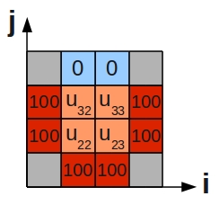
This describes purely diffusive phenomena and can give us the steady state temperature over a 2D plate, three sides of which are held at 100°C, while the fourth is held at 0°C. We have divided the plate into a number of grid cells:
Using the central difference approximation to a 2nd differential that we derived in the last section, we can rewrite the differential equation as a difference equation:
- [math]\displaystyle{ \frac{\partial^2u}{\partial x^2} + \frac{\partial^2u}{\partial y^2} \approx \frac{1}{h^2}(u^j_{i+1} -2u^j_i +u^j_{i-1}) + \frac{1}{k^2}(u^{j+1}_i -2u^j_i +u^{j-1}_i) }[/math]
where h is the grid spacing in the i-directions and k is the spacing the j-direction. If we set [math]\displaystyle{ h=k }[/math], then:
- [math]\displaystyle{ u^j_{i+1} + u^j_{i-1} + u^{j+1}_i + u^{j-1}_i - 4u^j_i = 0 }[/math]
solving for [math]\displaystyle{ u^j_i }[/math]:
- [math]\displaystyle{ u^j_i = \frac{1}{4}(u^j_{i+1} + u^j_{i-1} + u^{j+1}_i + u^{j-1}_i) }[/math]
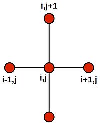
Note that this last equation says--quite intuitively--that the value at the central grid point is equal to the average of its four neighbours. We can draw a picture of the stencil needed to compute the value:
Placing the stencil on the 4 grid cells on the inner region (orange) in turn, we generate the following 4 difference equations:
- [math]\displaystyle{ \begin{alignat}{5} -4u_{22} & + u_{32} & + u_{23} & + 100 & + 100 & = 0 \\ -4u_{32} & + 0 & + u_{33} & + u_{22} & + 100 & = 0 \\ -4u_{23} & + u_{33} & + 100 & + 100 & + u_{22} & = 0 \\ -4u_{33} & + 0 & + 100 & + u_{23} & + u_{32} & = 0 \\ \end{alignat} }[/math]
This system of equations can be written in matrix form:
- [math]\displaystyle{ \begin{bmatrix}-4 & 1 & 1 & 0\\1 & -4 & 0 & 1\\1 & 0 & -4 & 1\\0 & 1 & 1 & -4\end{bmatrix} \begin{bmatrix}u_{22}\\u_{32}\\u_{23}\\u_{33}\end{bmatrix} = \begin{bmatrix}-200\\-100\\-200\\-100\end{bmatrix} }[/math]
Which may be summarised as the vector equation, Ax=b, which can be efficiently & conveniently solved using a library linear algebra routines, such as LAPACK, PETSc or PLASMA.
Parabolic Equations: Forward Euler
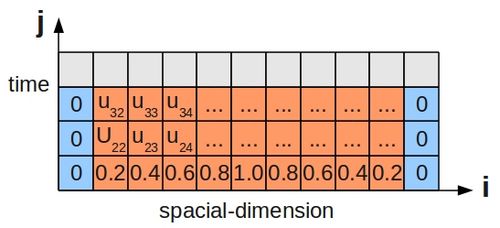
One example of a parabolic equation is the 1D heat equation, which describes the evolution of temperature at various points in a thin, insulated bar over time. Imagine such a bar where the ends are kept at 0°C:
Since this scenario involves the passage of time, just stating the boundary conditions is not enough, and we must also specify some initial condition for the temperature along the bar's length. This is shown below for a bar divided up into grid cells, as before:
The 1D heat equation is:
- [math]\displaystyle{ \frac{\partial u}{\partial t}=\alpha \frac{\partial^2u}{\partial x^2} }[/math]
where [math]\displaystyle{ \alpha }[/math]--the thermal diffusivity--is set to 1 for simplicity. One way to rewrite this as a difference equation (using a forward difference for the LHS and a central difference for the RHS) is:
- [math]\displaystyle{ \frac{u^{j+1}_i - u^j_i }{k} = \frac{u^j_{i+1} - 2u^j_i + u^j_{i-1}}{h^2} }[/math]
and rearrange to solve for [math]\displaystyle{ u^{j+1}_i }[/math]:
- [math]\displaystyle{ u^{j+1}_i = u^j_i + r(u^j_{i+1} - 2u^j_i + u^j_{i-1}) }[/math]
- [math]\displaystyle{ u^{j+1}_i = ru^j_{i+1} + (1- 2r)u^j_i + ru^j_{i-1} }[/math]
where:
[math]\displaystyle{ r=\frac{k}{h^2} }[/math]
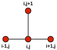
This time, we see that the appropriate stencil is:
If we set [math]\displaystyle{ h=\frac{1}{10} }[/math] and [math]\displaystyle{ k=\frac{1}{1000} }[/math], then [math]\displaystyle{ r=\frac{1}{10} }[/math], and the equation becomes:
- [math]\displaystyle{ u^{j+1}_i = u^j_i + \frac{1}{10}(u^j_{i+1} - 2u^j_i + u^j_{i-1}) }[/math]
- [math]\displaystyle{ u^{j+1}_i = \frac{1}{10}(u^j_{i+1} + 10u^j_i - 2u^j_i + u^j_{i-1}) }[/math]
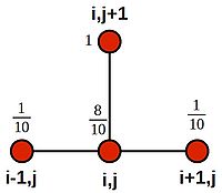
- [math]\displaystyle{ u^{j+1}_i = \frac{1}{10}(u^j_{i+1} + 8u^j_i + u^j_{i-1}) }[/math]
Which we can illustrate using weightings on the stencil nodes:
Forward Euler is as an explicit method, as one unknown value ([math]\displaystyle{ u^{j+1}_i }[/math]) is expressed directly in terms of known values (all values of u at time j are known).
We could implement a simple marching algorithm, where we centre the stencil over a set of known values at time j, and may calculate the unknown temperature for grid cell i at time j+1. However, it would be better to group together all the calculations for a particular time step into a system of simultaneous equations and then re-write in matrix form:
- [math]\displaystyle{ \begin{bmatrix} 0.1 & 0.8 & 0.1 & 0 & 0 & \cdots & 0 \\ 0 & 0.1 & 0.8 & 0.1 & 0 & \cdots & 0 \\ \vdots & & & & & & \vdots \\ & & \cdots & 0 & 0.1 & 0.8 & 0.1 \\ \end{bmatrix} \times \begin{bmatrix}0 \\ 0.2 \\ 0.4 \\ \vdots \\ 0.2 \\ 0 \end{bmatrix} = \begin{bmatrix}u_{22} \\ \vdots \\ u_{{m-1},{n-1}} \end{bmatrix} }[/math]
as the computational efficiency of a matrix vector multiplication will be hard to better.
Note that we can write the above piece of linear algebra in a general form:
- [math]\displaystyle{ \begin{bmatrix} r & 1-2r & r & 0 & 0 & \cdots & 0 \\ 0 & r & 1-2r & r & 0 & \cdots & 0 \\ \vdots & & & & & & \vdots \\ & & \cdots & 0 & r & 1-2r & r \\ \end{bmatrix} \times \begin{bmatrix}0 \\ 0.2 \\ 0.4 \\ \vdots \\ 0.2 \\ 0 \end{bmatrix} = \begin{bmatrix}u_{22} \\ \vdots \\ u_{{m-1},{n-1}} \end{bmatrix} }[/math]
Parabolic Equations: Backward Euler
An alternative way to formulate our finite difference is to use a backward difference on the LHS, keeping the central difference on the RHS, but shifting the time index to j+1, so as maintain a backward difference on the LHS:
- [math]\displaystyle{ \frac{u^{j+1}_i - u^j_i }{k} = \frac{u^{j+1}_{i+1} - 2u^{j+1}_i + u^{j+1}_{i-1}}{h^2} }[/math]
- [math]\displaystyle{ u^{j+1}_i - u^j_i = \frac{k}{h^2}(u^{j+1}_{i+1} - 2u^{j+1}_i + u^{j+1}_{i-1}) }[/math]
- [math]\displaystyle{ u^{j+1}_i - u^j_i = r(u^{j+1}_{i+1} - 2u^{j+1}_i + u^{j+1}_{i-1}) }[/math]
- [math]\displaystyle{ u^{j+1}_i - u^j_i = ru^{j+1}_{i+1} - 2ru^{j+1}_i + ru^{j+1}_{i-1} }[/math]
- [math]\displaystyle{ u^{j+1}_i - ru^{j+1}_{i+1} + 2ru^{j+1}_i - ru^{j+1}_{i-1} = u^j_i }[/math]
- [math]\displaystyle{ u^j_i = - ru^{j+1}_{i+1} + (1 + 2r)u^{j+1}_i - ru^{j+1}_{i-1} }[/math]
Parabolic Equations: Crank-Nicolson
The Forward Euler scheme has the benefit of simplicity, but is unstable for large time steps. The CFL (Courant–Friedrichs–Lewy) condition states that the following must hold:
- [math]\displaystyle{ r=\frac{k}{h^2} \le 0.5 }[/math]
for stability.
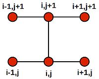
An alternative method to solve the 1D heat equation is to create a finite difference equation using the Crank-Nicolson stencil:
The stencil relates to an average of both the forward and backward Euler methods. The resulting difference equation is:
- [math]\displaystyle{ \frac{u^{j+1}_i - u^j_i}{k} = \frac{1}{2}(\frac{u^{j+1}_{i+1} - 2u^{j+1}_{i} + u^{j+1}_{i-1}}{h^2} + \frac{u^j_{i+1} - 2u^j_i + u^j_{i-1}}{h^2}). }[/math]
Which we may rearrange to become:
- [math]\displaystyle{ u^{j+1}_i - u^j_i = \frac{1}{2}\frac{k}{h^2}(u^{j+1}_{i+1} - 2u^{j+1}_i + u^{j+1}_{i-1} + u^j_{i+1} - 2u^j_i + u^j_{i-1}) }[/math]
- [math]\displaystyle{ 2(u^{j+1}_i - u^j_i) = r(u^{j+1}_{i+1} - 2u^{j+1}_i + u^{j+1}_{i-1} + u^j_{i+1} - 2u^j_i + u^j_{i-1}) }[/math],
where [math]\displaystyle{ r=\frac{k}{h^2} }[/math].
Collecting the unknowns (values of u at the next timestep, i+1) to the LHS and the knowns (values of u at current timestep, j), we get:
- [math]\displaystyle{ 2u^{j+1}_i + 2ru^{j+1}_i - ru^{j+1}_{i+1} - ru^{j+1}_{i-1} = 2u^j_i +ru^j_{i+1} -2ru^j_i + ru^j_{i-1} }[/math]
- [math]\displaystyle{ (2+2r)u^{j+1}_i - ru^{j+1}_{i+1} - ru^{j+1}_{i-1} = (2-2r)u^j_i +ru^j_{i+1} + ru^j_{i-1} }[/math].
If we choose [math]\displaystyle{ h=1/10 }[/math] and [math]\displaystyle{ k=1/100 }[/math] (note that the time-step is 10x larger than than chosen for the forward Euler example), then [math]\displaystyle{ r=1 }[/math], and we get:
- [math]\displaystyle{ -u_{i-1}^{j+1} +4u_i^{j+1} -u_{i+1}^{j+1} = u_{i-1}^j + u_{i+1}^j }[/math].
We can create a system of linear equations for all the cells j along the bar at a given time step i. We will have j unknowns and j equations. Then we can again translate into matrix notation and solve using a library linear algebra routines. Then we advance the time step and repeat the process, solving another system of equations. Compared the the forward Euler method, we must do more work at each time step to solve this system, but we may take larger time steps and the solution will still remain stable. For many problems, the Crank-Nicolson method is preferable.
Other Ways to Create Difference Equations
We have looked at the finite difference approach here, but other approaches exist, such as finite element and finite volume methods exist. Each approach has its pros and cons.
