NumericPython

numpy: An intro to some handy array tools in Python

A Quick Introduction to Python

Python is a high-level scripting language than can prove useful in a number of situations. On this page, we will mostly be looking at the array processing functions available through it's numpy package. However, we'll start with a little taster of the core language by way of an introduction. Python has lots to offer to the scientific programmer, through the routines contained within it's Scientific and numpy packages (offering a possible alternative to Matlab, IDL or R, for example), as well as it's visualisation tools. Python can also act as a flexible front-end to your Fortran or C routines. If you would like a more complete introduction to the language, there are a number of very good online tutorials (such as [1], for example), and also some good books by O'Reilly and New Riders, to name a couple. Python is freely available (and by that I mean gratis, at no cost) for Linux, Mac and Windows.

Getting Started with an Interactive Session

You can write scripts or start up the Python interpreter for an interactive session. We'll make a start interactively and move on to writing scripts later. At the Linux command line, you can invoke the interpreter by just typing:

python

and you should see something similar to:

Python 2.4.3 (#1, Jan 21 2009, 01:11:33) 
[GCC 4.1.2 20071124 (Red Hat 4.1.2-42)] on linux2
Type "help", "copyright", "credits" or "license" for more information.
>>> 

where we can type at the >>> prompt. To exit the interpreter, type Ctrl-D (i.e. the control key and D. Lower case is fine.)

OK, great! We're out of the starting gate. Let's get into our stride.

First, let's set a variable to a message. For example:

>>> message = "Hello, Gethin!"

Then type:

>>> print message

and, gratifyingly , I get:

hello, Gethin!

Python can, of course, do arithmetic, logic and all that good stuff. Just as an example, you could try some of the following:

>>> print 39 + 1

>>> print 2.2 * 3.3

>>> pi = 22/7
>>> print pi

>>> pi = 22.0/7.0
>>> print pi

>>> a=a=1.5+0.5j
>>> print a.real
...
>>> print a.imag

>>> if len(message) > 10:
...     print "message has more than 10 characters"
... 

You'll have to throw in a tab and hit enter a couple of times for the last one. And notice the good-old integer division gotcha in the approximation of pi.

Some Higher-Level Features

In the preamble, we mentioned that Python is a high-level language. What does that mean, exactly? Well, Python has some rather powerful data-types, such as lists and hash-tables aka 'dictionaries' built in, and also provides a rich language for manipulating the data-types that you are used to seeing in lower-level languages such as C and Fortran.

For example, the eagle-eyed will have spotted in the previous examples that we could ask the length a character string--straight off the bat. No need to write a counting routine ourselves:

>>> print len(message)

We also take slices of our character string. In my case

>>> print message[:5]

elicits:

hello

An example of a list is:

>>> shopping = ['bread', 'marmalade', 'milk', 'tea']

and we can enquire about the length of that using the same function as before:

>>> len(shopping)

A list object comes with a number of handy methods built in. For example we could type:

>>> shopping.append("butter")
>>> print shopping

and even:

>>> shopping.reverse()
>>> print shopping

or

>>> shopping.sort()
>>> print shopping

Arrays in numpy

OK, we could spend quite a while getting to grips with all of Python's myriad features, but we'll move onto looking at numerical features and arrays in particular. To do this we will load a package. You can do this by typing:

from numpy import *

Now that we have access to the package, let's create an array. Note that a numpy array is an objects of a different type to an intrinsic array in Python. A simple approach is to use the array function. For example we might enter:

>>> a = array([[1.0, 0.0, 0.0],[0.0, 1.0, 0.0],[0.0, 0.0, 1.0]])
>>> print a

Given an array, we may enquire about it's shape:

>>> print a.shape

and we are told that it is a 2-dimensional array (i.e. an array of rank 2) and that the length of both dimensions is 3:

(3, 3)

Should we so desire, we could re-shape the array. One way to do this is to to set it's shape attribute directly:

>>> a.shape = (1,9)
>>> print a

We can also apply operators to array objects. For example:

>>> a = a * 9
>>> print a

Note, however, that most operations on numpy arrays are done element-wise, which may be different to a linear algera operation that you were expecting. We will return to linear algebra operations in a later section.

More Interesting

x = arange(-5,10)
y = arange(-4,11)
z1 = sqrt(add.outer(x**2,y**2))
Z = sin(z1)/z1 

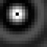
If you have the NumTut package available, then you can simply type:

from NumTut import *
view(Z)

and you should get a window similar to:

A grey-scale map of the sinc function

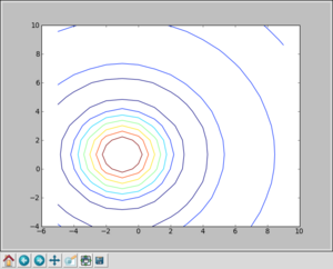
Otherwise, we can use the matplotlib package:

import matplotlib.pyplot as plt
from pylab import meshgrid
X, Y = meshgrid(x,y)
plt.figure()
plt.contour(X,Y,Z)
plt.show()

and you should get a window similar to:

A contour map of the sinc function